Transient mass diffusion

Read Transient mass diffusion as text

Download slides PDFDownload notes PDF

Slides by Shah (n.d.): view or download the slides.

1 Errata

• Slide 10 places the transformed finite-wall boundary condition at infinity. Apply it at the wall surface

  Θ(𝐿,𝑡)=0$$\Theta(L,t)=0$$

  The finite wall ends at 𝑥 =𝐿$x=L$.

• Slide 11 gives 𝑐𝐴 −𝑐𝐴0$c_A-c_{A0}$ as the normalized numerator and includes a stray 𝑥$x$ in the exponential decay factor. Use 𝑐𝐴 −𝑐𝐴𝑠$c_A-c_{As}$ in the numerator. With the slide’s full wall thickness 𝐿$L$, use the decay factor

  exp⁡(−𝑛2𝜋2𝐷𝐴𝐵𝑡𝐿2)$$\exp\left(-\frac{n^2\pi^2D_{AB}t}{L^2}\right)$$

• Slide 22 incorrectly groups the large-argument approximation. Use

  erf⁡(𝜂)≃1−𝑒−𝜂2𝜂√𝜋$$\operatorname{erf}(\eta)\simeq1-\frac{e^{-\eta^2}}{\eta\sqrt\pi}$$

  The printed grouping incorrectly divides the whole expression by 𝜂$\eta$.

• The deposition diagrams on slides 24 to 26 show a reaction that does not conserve oxygen. The printed reactants contain six oxygen atoms, while the products contain two. Use the balanced oxide-reduction step in the physical setup. The diffusion calculation starts with the maintained phosphorus surface concentration and does not use the erroneous reaction.

2 Reading list

• Bird et al. (2006), chapter 18.
• Geankoplis (2003), chapter 6.
• Welty et al. (2001), chapter 25.

Use molar flux in mol m−2 s−1$\mathrm{mol\,m^{-2}\,s^{-1}}$ and concentration in mol m−3$\mathrm{mol\,m^{-3}}$, unless an example specifies mass or atomic concentration.

3 Choose a time-dependent diffusion model

Given conditions	Model and checks
Slowly shrinking reacting body	Use a pseudo-steady surrounding profile with a moving-boundary inventory, Eq. 8.
Finite body, nearly uniform interior	Test 𝑘𝑐(𝑉/𝐴𝑠)/𝐷𝐴𝐵 ≤0.1$k_c(V/A_s)/D_{AB}\le0.1$ on a common concentration basis before using a lumped balance.
Finite body with internal gradients	Use half-thickness or radius in the Fourier and Biot numbers, Eq. 14; select the matching geometry and surface condition.
Early diffusion into a deep medium	Use the semi-infinite step solution; check penetration depth against the actual body dimension.
Reaction distributed within the body	Add a volume reaction term; the source-free diffusion solutions here no longer apply unchanged.

4 Pseudo steady state analysis

Pseudo steady state

An approximation that neglects accumulation in a rapidly adjusting transport region while a slower boundary or system state changes with time. Its validity requires separated transport and system time scales.

4.1 Coal particle burning

A spherical carbon particle of current radius 𝑅$R$ burns in an effectively infinite gas. Oxygen diffuses inward, and carbon monoxide and carbon dioxide diffuse outward. The source assumes the product split

3C(s)+2.5O2(g)⟶2CO2(g)+CO(g)$$3\mathrm{C(s)}+2.5\mathrm{O_2(g)} \longrightarrow 2\mathrm{CO_2(g)}+\mathrm{CO(g)}$$(1)

The atomic balance is correct. This particular split is an input to the model, not a universal combustion law. We assume instantaneous surface reaction, no homogeneous reaction in the gas, constant temperature, total molar concentration 𝑐$c$ and effective oxygen-mixture diffusivity 𝐷$D$. The actual four-species problem generally requires multicomponent diffusion. Replacing it with one effective 𝐷$D$ is an additional approximation.

The gas establishes its profile on a time scale 𝑅2/𝐷$R^2/D$. Treating that profile as steady at each instant is justified only when this time is much shorter than the particle shrinkage time. For a radius of 100$100$ micrometres and 𝐷 =10−4$D=10^{-4}$ m² s⁻¹ the relaxation scale is 10−4$10^{-4}$ s. This estimate alone does not determine burnout time; density, gas concentration and kinetics also matter. Fast kinetics must be checked independently.

Figure 1: Oxygen diffuses inward while gaseous products diffuse outward. Positive radial flux points outward.

Spherical symmetry removes angular derivatives. No gas-phase reaction removes the source term. Pseudo steady state removes gas accumulation, so continuity reduces to

1𝑟2𝑑𝑑𝑟(𝑟2𝑁𝑂2,𝑟)=0,𝑟2𝑁𝑂2,𝑟=𝐶$$\frac{1}{r^2}\frac{d}{dr}(r^2N_{O_2,r})=0, \qquad r^2N_{O_2,r}=C$$(2)

The integration constant 𝐶$C$ has units mol s⁻¹. It is 𝑟2𝑁$r^2N$, rather than flux itself, that is constant. The molar rate crossing a sphere is 4𝜋𝐶$4\pi C$. Oxygen flux is negative because the positive coordinate points outward. Surface stoichiometry and stagnant nitrogen give

𝑁𝐶𝑂2,𝑟=−0.8𝑁𝑂2,𝑟𝑁𝐶𝑂,𝑟=−0.4𝑁𝑂2,𝑟𝑁𝑁2,𝑟=0𝑁tot,𝑟=−0.2𝑁𝑂2,𝑟$$\begin{aligned} N_{CO_2,r}&=-0.8N_{O_2,r}\\ N_{CO,r}&=-0.4N_{O_2,r}\\ N_{N_2,r}&=0\\ N_{\mathrm{tot},r}&=-0.2N_{O_2,r} \end{aligned}$$(3)

Three moles of gas leave for every 2.5 moles of oxygen consumed. Consequently the total molar flux points outward and opposes inward oxygen diffusion. Nitrogen has zero total flux, although its diffusion and mixture transport need not separately vanish.

The effective mixture flux law and Eq. 3 yield

𝑁𝑂2,𝑟=−𝑐𝐷𝑑𝑦𝑑𝑟+𝑦𝑁tot,𝑟𝑁𝑂2,𝑟=−𝑐𝐷1+0.2𝑦𝑑𝑦𝑑𝑟𝐶=−𝑐𝐷𝑟21+0.2𝑦𝑑𝑦𝑑𝑟$$\begin{aligned} N_{O_2,r}&=-cD\frac{dy}{dr}+yN_{\mathrm{tot},r}\\ N_{O_2,r}&=-\frac{cD}{1+0.2y}\frac{dy}{dr}\\ C&=-\frac{cDr^2}{1+0.2y}\frac{dy}{dr} \end{aligned}$$(4)

Here 𝑦 =𝑦𝑂2$y=y_{O_2}$. The boundary conditions are 𝑦(𝑅) =0$y(R)=0$, from instantaneous reaction, and 𝑦(∞) =𝑦∞ =0.21$y(\infty)=y_\infty=0.21$, from ambient air. Separating Eq. 4 gives

𝐶∫∞𝑅𝑑𝑟𝑟2=−𝑐𝐷∫𝑦∞0𝑑𝑦1+0.2𝑦𝐶𝑅=−5𝑐𝐷ln⁡(1+0.2𝑦∞)𝑁𝑂2,𝑟(𝑅)=−5𝑐𝐷𝑅ln⁡(1.042)$$\begin{aligned} C\int_R^\infty\frac{dr}{r^2} &=-cD\int_0^{y_\infty}\frac{dy}{1+0.2y}\\ \frac{C}{R}&=-5cD\ln(1+0.2y_\infty)\\ N_{O_2,r}(R)&=-\frac{5cD}{R}\ln(1.042) \end{aligned}$$(5)

The logarithm is dimensionless. Its coefficient 5ln⁡(1.042) =0.20571$5\ln(1.042)=0.20571$ replaces the pure-diffusion coefficient 0.21$0.21$. The outward mixture motion lowers the inward flux magnitude by about 2.04 percent.

The remaining concentration profile follows by integrating only to radius 𝑟$r$:

ln⁡(1+0.2𝑦(𝑟))=ln⁡(1.042)(1−𝑅𝑟)$$\ln(1+0.2y(r)) =\ln(1.042)\left(1-\frac{R}{r}\right)$$(6)

It satisfies both endpoints, and differentiating it recovers Eq. 4. Carbon consumption rate, written ˙𝑛𝐶$\dot n_C$ in mol s⁻¹, is positive:

˙𝑛𝐶=32.5 4𝜋𝑅2∣𝑁𝑂2,𝑟(𝑅)∣=24𝜋𝑐𝐷ln⁡(1.042)𝑅$$\dot n_C =\frac{3}{2.5}\,4\pi R^2|N_{O_2,r}(R)| =24\pi cD\ln(1.042)R$$(7)

With carbon density 𝜌𝐶$\rho_C$ in kg m⁻³ and molar mass 𝑀𝐶$M_C$ in kg mol⁻¹, the shrinking solid balance is

𝜌𝐶𝑀𝐶4𝜋𝑅2𝑑𝑅𝑑𝑡=−˙𝑛𝐶𝑅𝑑𝑅𝑑𝑡=−6𝑐𝐷𝑀𝐶𝜌𝐶ln⁡(1.042)𝑅2(𝑡)=𝑅20−𝐾𝑡𝐾=12𝑐𝐷𝑀𝐶𝜌𝐶ln⁡(1.042)$$\begin{aligned} \frac{\rho_C}{M_C}4\pi R^2\frac{dR}{dt} &=-\dot n_C\\ R\frac{dR}{dt} &=-\frac{6cDM_C}{\rho_C}\ln(1.042)\\ R^2(t)&=R_0^2-Kt\\ K&=\frac{12cDM_C}{\rho_C}\ln(1.042) \end{aligned}$$(8)

The coefficient 𝐾$K$ has units m² s⁻¹. Burnout occurs at 𝑡𝑏 =𝑅20/𝐾$t_b=R_0^2/K$. This is a radius-squared law, and doubling the initial radius quadruples the model burnout time. Its use ends if surface kinetics, gas reaction, changing composition or temperature invalidates the assumptions.

Worked coal burnout model

For the reaction and air composition above, find the particle radius and burnout time in terms of 𝑅0$R_0$, 𝑐$c$, 𝐷$D$, 𝜌𝐶$\rho_C$ and 𝑀𝐶$M_C$. Quantify the flux correction relative to pure diffusion.

Calculation and answer

Data

Quantity	Value
Initial particle radius	𝑅0$R_0$
Gas total molar concentration	𝑐$c$
Effective oxygen diffusivity	𝐷$D$
Carbon density	𝜌𝐶$\rho_C$
Carbon molar mass	𝑀𝐶$M_C$
Ambient oxygen mole fraction	𝑦𝑂2,∞ =0.21$y_{O_2,\infty}=0.21$
Reaction stoichiometry	2.5 mol oxygen consumed per 3 mol carbon

Assumptions

• Spherical particle with uniform solid density.
• Pseudo steady diffusion in the surrounding gas.
• Instantaneous surface reaction and no gas-phase reaction.
• Constant temperature, total concentration and effective diffusivity.

Calculations

The steady gas calculation supplies the oxygen flux at each current radius. Writing Eq. 5 for the inward magnitude gives

∣𝑁𝑂2,𝑟(𝑅)∣=5𝑐𝐷𝑅ln⁡(1+0.2𝑦∞)$$|N_{O_2,r}(R)|=\frac{5cD}{R}\ln(1+0.2y_\infty)$$

Substituting the ambient mole fraction gives

∣𝑁𝑂2,𝑟(𝑅)∣=5𝑐𝐷𝑅ln⁡(1.042)=0.20571𝑐𝐷𝑅$$|N_{O_2,r}(R)|=\frac{5cD}{R}\ln(1.042) =0.20571\frac{cD}{R}$$

Multiply the oxygen rate by the stoichiometric carbon-to-oxygen ratio:

˙𝑛𝐶=32.5 4𝜋𝑅2∣𝑁𝑂2,𝑟(𝑅)∣=24𝜋𝑐𝐷ln⁡(1.042)𝑅$$\dot n_C=\frac{3}{2.5}\,4\pi R^2|N_{O_2,r}(R)| =24\pi cD\ln(1.042)R$$

The carbon inventory is

𝑛𝐶=(𝜌𝐶𝑀𝐶)4𝜋𝑅33.$$n_C=\left(\frac{\rho_C}{M_C}\right)\frac{4\pi R^3}{3}.$$

Its decrease equals the positive consumption rate:

𝜌𝐶𝑀𝐶4𝜋𝑅2𝑑𝑅𝑑𝑡=−24𝜋𝑐𝐷ln⁡(1.042)𝑅$$\frac{\rho_C}{M_C}4\pi R^2\frac{dR}{dt} =-24\pi cD\ln(1.042)R$$

Cancel a factor of radius and integrate from 𝑅0$R_0$ at zero time to 𝑅$R$ at time 𝑡$t$:

∫𝑅𝑅0𝑅 𝑑𝑅=−6𝑐𝐷𝑀𝐶𝜌𝐶ln⁡(1.042)∫𝑡0𝑑𝑡$$\int_{R_0}^{R}R\,dR =-\frac{6cDM_C}{\rho_C}\ln(1.042)\int_0^t dt$$

Thus 𝑅2 =𝑅20 −𝐾𝑡$R^2=R_0^2-Kt$, with

𝐾=12𝑐𝐷𝑀𝐶ln⁡(1.042)𝜌𝐶.$$K=\frac{12cDM_C\ln(1.042)}{\rho_C}.$$

The dimensions of 𝐾$K$ are m2 s−1$\mathrm{m^{2}\,s^{-1}}$, as required for a radius-squared decay law.

Without outward mixture flow, the oxygen flux magnitude would be 0.21𝑐𝐷/𝑅$0.21cD/R$. The relative reduction is

1−0.205710.21=0.02043$$1-\frac{0.20571}{0.21}=0.02043$$

The outward product flow therefore reduces the oxygen supply by 2.04 percent. Doubling 𝑅0$R_0$ quadruples burnout time within this model.

Answer

The radius and burnout time are

𝑅(𝑡)=√𝑅20−𝐾𝑡,𝐾=0.49370𝑐𝐷𝑀𝐶𝜌𝐶$$R(t)=\sqrt{R_0^2-Kt},\qquad K=0.49370\frac{cDM_C}{\rho_C}$$𝑡𝑏=𝜌𝐶𝑅200.49370𝑐𝐷𝑀𝐶$$t_b=\frac{\rho_CR_0^2}{0.49370cDM_C}$$

The radius expression applies for 0 ≤𝑡 ≤𝑡𝑏$0\leq t\leq t_b$. The oxygen flux is 2.04 percent smaller than the pure-diffusion estimate. No numerical burnout time is determined without the carbon density and operating gas properties.

A coal particle shrinks while its surrounding gas concentration field adjusts rapidly. When is a pseudo steady gas model justified?

• Whenever the particle radius is changing.
• Only when the particle radius is exactly constant.
• When gas diffusion adjusts much faster than the particle shrinks. ✓
• Whenever surface reaction is fast, regardless of gas diffusion time.

Explanation

The gas diffusion time is of order

𝑡gas∼𝑅2𝐷$$t_{\mathrm{gas}}\sim\frac{R^2}{D}$$

It must be much shorter than the time over which the particle radius changes appreciably. Then the gas field can be treated as steady at each slowly changing radius. A fast surface reaction alone does not establish this separation of times.

5 Unsteady-state diffusion in a finite medium

5.1 Equation and boundary conditions

For a stationary medium, negligible bulk transport, no reaction and one-dimensional constant-property diffusion, species continuity becomes Fick’s second law:

∂𝑐𝐴∂𝑡=𝐷𝐴𝐵∂2𝑐𝐴∂𝑥2$$\frac{\partial c_A}{\partial t} =D_{AB}\frac{\partial^2c_A}{\partial x^2}$$(9)

Stationary solids and dilute solutes in stationary liquids can meet these assumptions. Equimolar counter-diffusion also removes total molar transport when the corresponding total-concentration model applies. Dilution alone does not remove imposed convection. These are reductions of continuity, not properties of every transient mixture.

The source begins with a wall of full thickness 𝐻$H$, exposed at both faces to the same prescribed surface concentration 𝑐𝐴𝑠$c_{As}$. Its initial concentration is uniformly 𝑐𝐴𝑖$c_{Ai}$. The conditions are

𝑐𝐴(𝑥,0)=𝑐𝐴𝑖$$c_A(x,0)=c_{Ai}$$

for 0 <𝑥 <𝐻$0<x<H$ and

𝑐𝐴(0,𝑡)=𝑐𝐴(𝐻,𝑡)=𝑐𝐴𝑠$$c_A(0,t)=c_A(H,t)=c_{As}$$

for 𝑡 >0$t>0$. The initially discontinuous face value represents an ideal step. Define

Θ=𝑐𝐴−𝑐𝐴𝑠𝑐𝐴𝑖−𝑐𝐴𝑠$$\Theta=\frac{c_A-c_{As}}{c_{Ai}-c_{As}}$$(10)

The symbol Θ$\Theta$ denotes a dimensionless concentration departure. Lower-case 𝜃$\theta$ is reserved for a dimensional temperature excess in the heat notes. The departure ratio in Eq. 10 goes from one initially to zero at equilibrium. Because the transformation is linear, Eq. 9 holds with Θ$\Theta$ replacing 𝑐𝐴$c_A$. Its conditions are Θ(𝑥,0) =1$\Theta(x,0)=1$, Θ(0,𝑡) =0$\Theta(0,t)=0$, and Θ(𝐻,𝑡) =0$\Theta(H,t)=0$.

5.2 Series solution and symmetry

Separation of variables sets Θ =𝑋(𝑥)𝑇(𝑡)$\Theta=X(x)T(t)$. Division by 𝐷𝐴𝐵𝑋𝑇$D_{AB}XT$ gives

𝑋′′𝑋=𝑇′𝐷𝐴𝐵𝑇=−𝜇2.$$\frac{X''}{X}=\frac{T'}{D_{AB}T}=-\mu^2.$$

Homogeneous face conditions select

𝑋𝑛=sin⁡(𝑛𝜋𝑥𝐻)$$X_n=\sin\left(\frac{n\pi x}{H}\right)$$

and temporal factors

exp⁡(−𝑛2𝜋2𝐷𝐴𝐵𝑡𝐻2).$$\exp\left(-\frac{n^2\pi^2D_{AB}t}{H^2}\right).$$

Expanding the initial value one in a sine series gives coefficient 4/(𝑛𝜋)$4/(n\pi)$ for odd 𝑛$n$ and zero for even 𝑛$n$. Thus

Θ(𝑥,𝑡)=4𝜋∑𝑛=1,3,5,…sin⁡(𝑛𝜋𝑥𝐻)𝑛 𝐸𝑛𝐸𝑛=exp⁡(−𝑛2𝜋2𝐷𝐴𝐵𝑡𝐻2)$$\begin{aligned} \Theta(x,t)&=\frac4\pi\sum_{n=1,3,5,\ldots} \frac{\sin\left(\frac{n\pi x}{H}\right)}{n}\,E_n\\ E_n&=\exp\left(-\frac{n^2\pi^2D_{AB}t}{H^2}\right) \end{aligned}$$(11)

Differentiating the series gives the molar flux

𝑁𝐴,𝑥=4𝐷𝐴𝐵𝐻(𝑐𝐴𝑠−𝑐𝐴𝑖)𝑆𝑆=∑𝑛=1,3,5,…cos⁡(𝑛𝜋𝑥𝐻)𝐸𝑛$$\begin{aligned} N_{A,x}&=\frac{4D_{AB}}{H}(c_{As}-c_{Ai})S\\ S&=\sum_{n=1,3,5,\ldots}\cos\left(\frac{n\pi x}{H}\right)E_n \end{aligned}$$(12)

At 𝑥 =𝐻/2$x=H/2$ every cosine is zero, so there is no flux through the symmetry plane. Higher modes decay faster than the first. The series represents the initial interior value in its limit at 𝑡 =0$t=0$; at the stepped faces it follows the imposed condition.

Mass Fourier number

The dimensionless time Fo𝑚 =𝐷𝐴𝐵𝑡/𝐿2$\mathrm{Fo}_m=D_{AB}t/L^2$, elapsed time divided by the species-diffusion time 𝐿2/𝐷𝐴𝐵$L^2/D_{AB}$. Use wall half-thickness or cylinder or sphere radius for the finite-body solutions here. It corresponds to the thermal Fourier number with 𝐷𝐴𝐵$D_{AB}$ replacing 𝛼$\alpha$.

The mass Fourier number indicates how far diffusion has progressed:

• For Fo𝑚 ≪1$\mathrm{Fo}_m\ll1$, the diffusion distance √𝐷𝐴𝐵𝑡$\sqrt{D_{AB}t}$ is small compared with 𝐿$L$. A semi-infinite model can describe early changes near an exposed surface if distant boundaries have little influence.
• For Fo𝑚 ∼1$\mathrm{Fo}_m\sim1$, diffusion has reached distances comparable to the body length. Finite geometry and the other boundaries matter.
• For Fo𝑚 ≫1$\mathrm{Fo}_m\gg1$, diffusion has had time to redistribute species throughout the body. A small external transfer coefficient can still delay equilibration with the surroundings.

The boundary condition and any external resistance determine how far equilibration has progressed. The wall example below gives 0.25 using half-thickness and 0.0625 using full thickness. That factor of four changes whether the stated one-term approximation is justified.

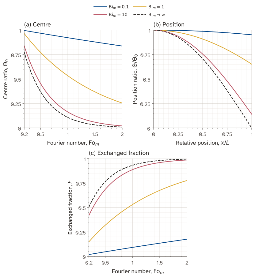
For charts and the following formulas, use half-thickness 𝐿 =𝐻/2$L=H/2$, centre coordinate

𝜉=𝑥−𝐻2𝐿$$\xi=\frac{x-\frac{H}{2}}{L}$$

and Fourier number Fo𝑚 =𝐷𝐴𝐵𝑡/𝐿2$\mathrm{Fo}_m=D_{AB}t/L^2$. Confusing full and half thickness changes the Fourier number by a factor of four. For a prescribed surface concentration the centre and spatial one-term solution is

Θ0≃4𝜋𝑒−𝜋2Fo𝑚4ΘΘ0≃cos⁡(𝜋𝜉2)$$\begin{aligned} \Theta_0&\simeq\frac4\pi e^{-\frac{\pi^2\mathrm{Fo}_m}{4}}\\ \frac{\Theta}{\Theta_0}&\simeq\cos\left(\frac{\pi\xi}{2}\right) \end{aligned}$$(13)

Here subscript zero means the centre value, not initial time. The omitted second mode decays nine times as fast. A one-term approximation is useful for Fo𝑚 ≳0.2$\mathrm{Fo}_m\gtrsim0.2$ using this half-thickness convention; it is an approximation, not an exact formula for all finite times.

A wall has full thickness 𝐻 =4$H=4$ mm and equal exposure at both faces. For its half-thickness Fourier number, use 𝐷 =10−9 m2 s−1$D=10^{-9}\ \mathrm{m^2\,s^{-1}}$ and 𝑡 =1000$t=1000$ s. What is Fo𝑚$\mathrm{Fo}_m$?

• 0.25$0.25$. ✓
• 0.0625$0.0625$.
• 0.50$0.50$.
• 4.0$4.0$.

Explanation

For equal exposure on both faces, use the half-thickness:

𝐿=𝐻2=0.002 m$$L=\frac{H}{2}=0.002\ \mathrm m$$

Thus,

Fo𝑚=𝐷𝑡𝐿2=10−9(1000)(0.002)2=0.25$$\mathrm{Fo}_m=\frac{Dt}{L^2}=\frac{10^{-9}(1000)}{(0.002)^2}=0.25$$

Using the full thickness would give a Fourier number four times smaller.

5.3 Groups used in the finite-body examples

Mass Biot number

The dimensionless resistance ratio Bi𝑚 =𝑘𝑐𝐿/𝐷𝐴𝐵$\mathrm{Bi}_m=k_cL/D_{AB}$, comparing internal species-diffusion resistance with external film resistance on the same concentration basis. Here 𝑘𝑐$k_c$ is expressed on the interior basis. It is the species counterpart of the thermal Biot number.

Although its algebra resembles Sherwood number, mass Biot uses the body’s internal diffusivity and length, while Sherwood uses the fluid diffusivity and transfer length.

• For Bi𝑚 ≪1$\mathrm{Bi}_m\ll1$, the external film offers most of the resistance. Internal diffusion keeps the concentration nearly uniform, so a lumped species balance may be appropriate.
• For Bi𝑚 ∼1$\mathrm{Bi}_m\sim1$, internal diffusion and external film transfer both matter. Retain the spatial diffusion equation and the film boundary condition.
• For Bi𝑚 ≫1$\mathrm{Bi}_m\gg1$, internal diffusion limits the response and large concentration gradients can develop. The surface is close to equilibrium with the external fluid, so a prescribed surface concentration can be a useful approximation.

For a lumped-model test, use 𝐿𝑐 =𝑉/𝐴𝑠$L_c=V/A_s$, with exposed area 𝐴𝑠$A_s$, and check 𝑘𝑐𝐿𝑐/𝐷𝐴𝐵 ≤0.1$k_cL_c/D_{AB}\le0.1$. The half-thickness or radius used by finite-body solutions gives a different numerical value for cylinders and spheres.

For 𝑘𝑐 =10−5 m s−1$k_c=10^{-5}\ \mathrm{m\,s^{-1}}$, 𝐿 =10−3 m$L=10^{-3}\ \mathrm m$ and 𝐷𝐴𝐵 =10−9 m2 s−1$D_{AB}=10^{-9}\ \mathrm{m^2\,s^{-1}}$, Bi𝑚 =10$\mathrm{Bi}_m=10$; a uniform interior is unjustified. Convert phase concentrations before comparing resistances, and retain half-thickness or radius for the stated solutions.

Partition coefficient

An equilibrium ratio of concentrations in two phases, for example

𝐾=𝑐∗𝐴,inside𝑐∗𝐴,outside.$$K=\frac{c_{A,\mathrm{inside}}^*}{c_{A,\mathrm{outside}}^*}.$$

It is dimensionless only when numerator and denominator use the same concentration units and basis. Its direction must be specified before converting a film coefficient.

With this convention, an outside-basis film coefficient becomes 𝑘𝑐,inside =𝑘𝑐,outside/𝐾$k_{c,\mathrm{inside}}=k_{c,\mathrm{outside}}/K$. Reversing the definition of 𝐾$K$ reverses the conversion. A mole-fraction equilibrium slope cannot be substituted for a concentration ratio without the corresponding conversion.

For finite-body solutions define a geometry length 𝐿𝑔$L_g$: wall half-thickness 𝐿$L$ for a two-sided wall, or radius 𝑅𝑏$R_b$ for a long cylinder or sphere. Reserve 𝐿𝑐 =𝑉/𝐴𝑠$L_c=V/A_s$ for the lumped-model test. The two lengths are related by

Geometry	𝐿𝑔$L_g$ for the finite-body solution	𝐿𝑐 =𝑉/𝐴𝑠$L_c=V/A_s$ for the lumped test
Two-sided wall of thickness 2𝐿$2L$	𝐿$L$	𝐿$L$
Long cylinder, with end transfer neglected	𝑅𝑏$R_b$	𝑅𝑏/2$R_b/2$
Sphere	𝑅𝑏$R_b$	𝑅𝑏/3$R_b/3$

Use the geometry length consistently in both groups:

Fo𝑚=𝐷𝐴𝐵𝑡𝐿2𝑔$$\mathrm{Fo}_m=\frac{D_{AB}t}{L_g^2}$$

Bi𝑚=𝑘𝑐𝐿𝑔𝐷𝐴𝐵$$\mathrm{Bi}_m=\frac{k_cL_g}{D_{AB}}$$(14)

Here Bi𝑚$\mathrm{Bi}_m$ is based on 𝐿𝑔$L_g$, not 𝑉/𝐴𝑠$V/A_s$. A sphere with 𝑘𝑐𝑅𝑏/𝐷𝐴𝐵 =0.30$k_cR_b/D_{AB}=0.30$ has a lumped-test value of 0.10. Do not use 0.10 in a sphere eigenvalue equation that expects the radius-based value 0.30. Here 𝑘𝑐$k_c$ is on the interior concentration basis. Convert an external-phase concentration using the partition relation before imposing its boundary condition. Prescribed surface concentration corresponds to infinite Bi. Use the matching heat-equation solution with 𝛼$\alpha$ replaced by 𝐷𝐴𝐵$D_{AB}$ and temperature departure replaced by concentration departure.

Using the same concentration basis inside and outside a body, Bi𝑚 =𝑘𝑐𝐿/𝐷𝐴𝐵 ≫1$\mathrm{Bi}_m=k_cL/D_{AB}\gg1$. Which interpretation is correct?

• The interior concentration must be uniform.
• Internal diffusion is instantaneous.
• The external film supplies most of the resistance.
• Diffusion inside the body offers much more resistance than the outside film. ✓

Explanation

On the same concentration basis, the ratio of internal to external resistance is of order

𝐿𝐷𝐴𝐵1𝑘𝑐=𝑘𝑐𝐿𝐷𝐴𝐵=Bi𝑚$$\frac{\frac{L}{D_{AB}}}{\frac{1}{k_c}}=\frac{k_cL}{D_{AB}}=\mathrm{Bi}_m$$

A large mass Biot number means that internal diffusion offers much more resistance than the external film. Concentration can vary substantially inside the body; a uniform interior is not justified.

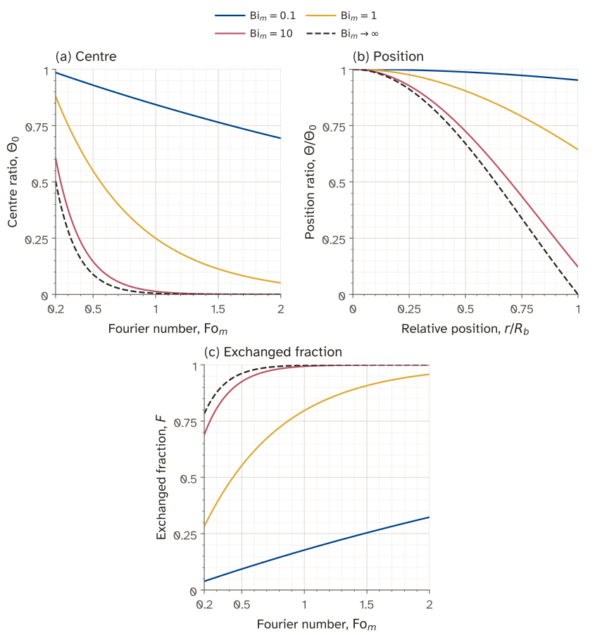
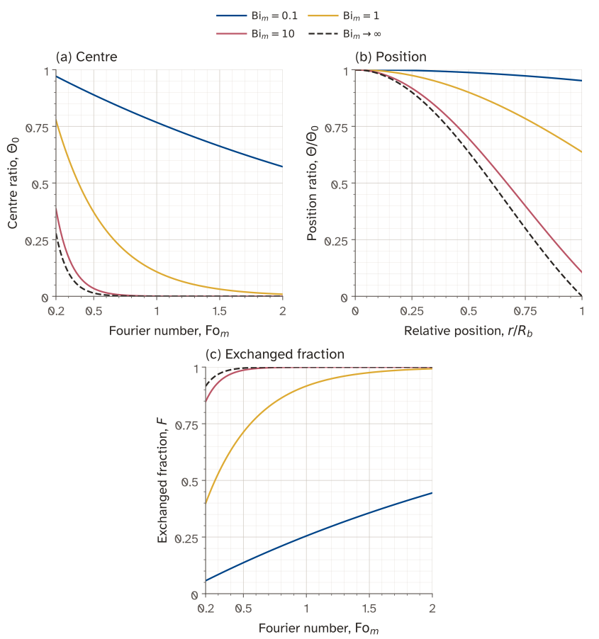
5.4 Application of Heisler charts

The following eigenvalue formulas supply the centre ratio, position correction and volume average needed for the classroom example (Çengel and Ghajar 2015).

For a plane wall measured from its centre, the convective boundary gives 𝜆tan⁡𝜆 =Bi𝑚$\lambda\tan\lambda=\mathrm{Bi}_m$. The lowest positive eigenvalue 𝜆1$\lambda_1$ and its amplitude are

𝐴1=4sin⁡𝜆12𝜆1+sin⁡(2𝜆1)Θ0≃𝐴1𝑒−𝜆21Fo𝑚ΘΘ0≃cos⁡(𝜆1𝜉)¯¯¯¯¯Θ≃Θ0sin⁡𝜆1𝜆1$$\begin{aligned} A_1&=\frac{4\sin\lambda_1}{2\lambda_1+\sin(2\lambda_1)}\\ \Theta_0&\simeq A_1e^{-\lambda_1^2\mathrm{Fo}_m}\\ \frac{\Theta}{\Theta_0}&\simeq\cos(\lambda_1\xi)\\ \bar\Theta&\simeq\Theta_0\frac{\sin\lambda_1}{\lambda_1} \end{aligned}$$(15)

The overbar means volume average. 𝐹 =1 −¯¯¯¯¯Θ$F=1-\bar\Theta$ is the fraction of the eventual total exchange completed, for either uptake or release. The original total-transfer charts use

Bi2𝑚Fo𝑚=𝑘2𝑐𝑡𝐷𝐴𝐵.$$\mathrm{Bi}_m^2\mathrm{Fo}_m=\frac{k_c^2t}{D_{AB}}.$$

At infinite Bi this coordinate diverges, so the finite one-term average is easier to use directly.

For an infinitely long cylinder of radius 𝑅𝑏$R_b$, radial diffusion has Bessel functions 𝐽0$J_0$ and 𝐽1$J_1$. These are mathematical functions, not the diffusive flux symbol 𝐽𝐴$J_A$. With 𝜁 =𝑟/𝑅𝑏$\zeta=r/R_b$, the eigenvalue condition and solution are

𝜆1𝐽1(𝜆1)=Bi𝑚𝐽0(𝜆1)𝐴1=2𝐽1(𝜆1)𝜆1[𝐽20(𝜆1)+𝐽21(𝜆1)]Θ0≃𝐴1𝑒−𝜆21Fo𝑚ΘΘ0≃𝐽0(𝜆1𝜁)¯¯¯¯¯Θ≃Θ02𝐽1(𝜆1)𝜆1$$\begin{aligned} \lambda_1J_1(\lambda_1)&=\mathrm{Bi}_mJ_0(\lambda_1)\\ A_1&=\frac{2J_1(\lambda_1)}{\lambda_1[J_0^2(\lambda_1)+J_1^2(\lambda_1)]}\\ \Theta_0&\simeq A_1e^{-\lambda_1^2\mathrm{Fo}_m}\\ \frac{\Theta}{\Theta_0}&\simeq J_0(\lambda_1\zeta)\\ \bar\Theta&\simeq\Theta_0\frac{2J_1(\lambda_1)}{\lambda_1} \end{aligned}$$(16)

For infinite Bi, 𝜆1 =2.40483$\lambda_1=2.40483$ and 𝐴1 =1.60197$A_1=1.60197$. A short cylinder also diffuses axially. Under separable initial and boundary conditions its solution is the product of a radial cylinder solution and an axial plane-wall solution. Whether end effects can be ignored depends on time and position as well as aspect ratio. The source’s length rule is a practical estimate, not a universal exact threshold.

For a sphere of radius 𝑅𝑏$R_b$, define 𝜁 =𝑟/𝑅𝑏$\zeta=r/R_b$. The eigenvalue condition is 1 −𝜆1cot⁡𝜆1 =Bi𝑚$1-\lambda_1\cot\lambda_1=\mathrm{Bi}_m$, and

𝐴1=4(sin⁡𝜆1−𝜆1cos⁡𝜆1)2𝜆1−sin⁡(2𝜆1)Θ0≃𝐴1𝑒−𝜆21Fo𝑚ΘΘ0≃sin⁡(𝜆1𝜁)𝜆1𝜁¯¯¯¯¯Θ≃3Θ0sin⁡𝜆1−𝜆1cos⁡𝜆1𝜆31$$\begin{aligned} A_1&=\frac{4(\sin\lambda_1-\lambda_1\cos\lambda_1)}{2\lambda_1-\sin(2\lambda_1)}\\ \Theta_0&\simeq A_1e^{-\lambda_1^2\mathrm{Fo}_m}\\ \frac{\Theta}{\Theta_0}&\simeq\frac{\sin(\lambda_1\zeta)}{\lambda_1\zeta}\\ \bar\Theta&\simeq3\Theta_0 \frac{\sin\lambda_1-\lambda_1\cos\lambda_1}{\lambda_1^3} \end{aligned}$$(17)

At the centre the position ratio has limiting value one. At infinite Bi, 𝜆1 =𝜋$\lambda_1=\pi$, 𝐴1 =2$A_1=2$, and

Θ0≃2𝑒−𝜋2Fo𝑚,𝐹≃1−3Θ0𝜋2$$\Theta_0\simeq2e^{-\pi^2\mathrm{Fo}_m}, \qquad F\simeq1-\frac{3\Theta_0}{\pi^2}$$(18)

Figure 2: One-term plane-wall diffusion solutions for the centre, position ratio and exchanged fraction.

Figure 3: One-term long-cylinder diffusion solutions for the centre, position ratio and exchanged fraction.

Figure 4: One-term spherical diffusion solutions for the centre, position ratio and exchanged fraction.

Drug capsule

A spherical drug capsule (0.652 cm diameter) has an initial concentration of 68.9 mg/cm3$^3$ Dramamine.

• What is the residual concentration of Dramamine at the centre of the spherical bead after 48 hours?

The capsule is intended to release the drug in the gastrointestinal system. Its nontoxic gelatinous material allows the drug to diffuse out gradually. The drug within the bead is the source of A; the surrounding fluid is the sink.

Data: 𝐷𝐴𝐵$D_{AB}$ (Dramamine in the gel matrix of the capsule) = 3 ×10−7 cm2/s$3\times10^{-7}\ \mathrm{cm^2/s}$ at body temperature of 37 °C$37\ \degree\mathrm{C}$.

Calculation and answer

Figure 5: Drug initially fills the spherical bead uniformly. It diffuses radially to a sink at the surface. Total release requires the concentration averaged over the whole bead.

The spherical diffusion model is the one shown in Figure 4. The maintained sink fixes the surface concentration, while the centre concentration is the requested unknown.

Data

Quantity	Value
Bead diameter	𝑑 =0.652 cm$d=0.652\ \mathrm{cm}$
Bead radius	𝑅𝑏 =0.326 cm$R_b=0.326\ \mathrm{cm}$
Initial drug concentration	𝐶𝑚𝑖 =68.9 mg cm−3$C_{mi}=68.9\ \mathrm{mg\,cm^{-3}}$
Drug diffusivity	𝐷 =3 ×10−7 cm2 s−1$D=3\times10^{-7}\ \mathrm{cm^2\,s^{-1}}$
Duration	𝑡 =48 h =172800 s$t=48\ \mathrm h=172800\ \mathrm s$
Body temperature	𝑇 =37 °C$T=37\ \degree\mathrm C$

Assumptions

• Spherical, stationary gel with constant radius.
• Uniform initial drug concentration.
• Well-stirred sink maintains zero surface concentration.
• No drug reaction within the gel.
• Constant diffusivity.

Calculations

The sink removes drug from the bead surface while internal diffusion supplies it from the centre. A prescribed surface concentration corresponds to infinite mass Biot number. First calculate the Fourier number using the radius:

Fo𝑚=𝐷𝑡𝑅2𝑏=3×10−7(172800)0.3262=0.48779$$\mathrm{Fo}_m=\frac{Dt}{R_b^2} =\frac{3\times10^{-7}(172800)}{0.326^2} =0.48779$$

The Fourier number exceeds 0.2, so the first spherical eigenmode is sufficient. For zero surface concentration the centre ratio is

Θ0=𝐶𝑚𝑐𝐶𝑚𝑖≃2𝑒−𝜋2Fo𝑚$$\Theta_0=\frac{C_{mc}}{C_{mi}}\simeq2e^{-\pi^2\mathrm{Fo}_m}$$

Substitution gives

Θ0≃2𝑒−𝜋2(0.48779)=0.016226$$\Theta_0\simeq2e^{-\pi^2(0.48779)}=0.016226$$

Multiply this ratio by the initial concentration to recover the centre concentration:

𝐶𝑚𝑐=𝐶𝑚𝑖Θ0=68.9(0.016226)=1.1180 mg cm−3$$C_{mc}=C_{mi}\Theta_0 =68.9(0.016226)=1.1180\ \mathrm{mg\,cm^{-3}}$$(19)

As an additional check on total release, the spherical volume-average ratio is ¯¯¯¯¯Θ ≃3Θ0/𝜋2$\bar\Theta\simeq3\Theta_0/\pi^2$. Hence

𝐹=1−¯¯¯¯¯Θ≃1−3(0.016226)𝜋2=0.99507$$F=1-\bar\Theta\simeq1-\frac{3(0.016226)}{\pi^2} =0.99507$$

The centre retains 1.62 percent of its initial concentration while only 0.493 percent of the initial drug remains in the entire bead. The centre has the largest residual concentration, so these two results have the expected order. Finite external resistance or swelling-dependent diffusivity requires a different model.

Answer

After 48 hours, the concentration at the centre is approximately

𝐶𝑚𝑐=1.12 mg cm−3$$C_{mc}=1.12\ \mathrm{mg\,cm^{-3}}$$

The corresponding additional estimate is 99.5 percent of the drug released.

A finite sphere releases solute to a sink. Which quantity determines the fraction of the eventual total release completed?

• One minus the centre concentration ratio.
• One minus the concentration departure ratio averaged over the whole sphere. ✓
• The surface concentration alone.
• The concentration at any arbitrarily chosen radius.

Explanation

Find how much solute remains by averaging concentration over the whole sphere. With the normalized departure used here,

𝐹=1−¯¯¯¯¯Θ$$F=1-\bar\Theta$$

The centre concentration describes only one position. It cannot be used in place of the volume average when calculating the amount released.

6 Unsteady-state diffusion in a semi-infinite medium

6.1 Conditions and similarity reduction

A stationary body occupies 𝑥 >0$x>0$ and starts uniformly at 𝑐𝐴𝑖$c_{Ai}$. At 𝑡 =0$t=0$ its surface is set to 𝑐𝐴𝑠$c_{As}$ and held there. With no reaction, no convection and constant diffusivity, Eq. 9 applies with

𝑐𝐴(𝑥,0)=𝑐𝐴𝑖,𝑐𝐴(0,𝑡)=𝑐𝐴𝑠,𝑐𝐴(∞,𝑡)=𝑐𝐴𝑖.$$\begin{aligned} c_A(x,0)&=c_{Ai},\\ c_A(0,t)&=c_{As},\\ c_A(\infty,t)&=c_{Ai}. \end{aligned}$$

A finite body approximates this model while the disturbance is shallow relative to its depth. An engineering depth estimate is 4√𝐷𝐴𝐵𝑡$4\sqrt{D_{AB}t}$, corresponding to less than 0.5 percent of the surface concentration change remaining. The condition 4√𝐷𝐴𝐵𝑡 <𝐿𝑐$4\sqrt{D_{AB}t}<L_c$ is Fo𝑚 <1/16$\mathrm{Fo}_m<1/16$, consistent with the earlier rough 0.05 threshold.

There is no imposed length in the infinite-depth problem. Diffusion supplies √𝐷𝐴𝐵𝑡$\sqrt{D_{AB}t}$, so set

𝜂=𝑥2√𝐷𝐴𝐵𝑡,𝑐𝐴(𝑥,𝑡)=𝑓(𝜂)$$\eta=\frac{x}{2\sqrt{D_{AB}t}}, \qquad c_A(x,t)=f(\eta)$$(20)

The factor two is a convention for the standard error function. The chain rule gives

∂𝑡𝑐𝐴=−𝜂2𝑡𝑓′∂2𝑥𝑐𝐴=14𝐷𝐴𝐵𝑡𝑓′′𝑓′′+2𝜂𝑓′=0$$\begin{aligned} \partial_t c_A&=-\frac{\eta}{2t}f'\\ \partial_x^2c_A&=\frac{1}{4D_{AB}t}f''\\ f''+2\eta f'&=0 \end{aligned}$$(21)

Set 𝑔 =𝑓′$g=f'$. Then 𝑔′/𝑔 = −2𝜂$g'/g=-2\eta$ gives 𝑔 =𝐵𝑒−𝜂2$g=B e^{-\eta^2}$, and a second integration gives

𝑓=𝐴+𝐵∫𝜂0𝑒−𝑢2 𝑑𝑢.$$f=A+B\int_0^\eta e^{-u^2}\,du.$$

Surface and far-field conditions determine 𝐴 =𝑐𝐴𝑠$A=c_{As}$ and

𝐵=2(𝑐𝐴𝑖−𝑐𝐴𝑠)√𝜋.$$B=\frac{2(c_{Ai}-c_{As})}{\sqrt\pi}.$$

Initial and far-field conditions both become the same 𝜂 →∞$\eta\to\infty$ limit. Thus three original conditions become two conditions for this second-order ODE.

erf⁡(𝜂)=2√𝜋∫𝜂0𝑒−𝑢2 𝑑𝑢𝑐𝐴−𝑐𝐴𝑖𝑐𝐴𝑠−𝑐𝐴𝑖=erfc⁡(𝜂)=1−erf⁡(𝜂)$$\begin{aligned} \operatorname{erf}(\eta)&=\frac2{\sqrt\pi}\int_0^\eta e^{-u^2}\,du\\ \frac{c_A-c_{Ai}}{c_{As}-c_{Ai}} &=\operatorname{erfc}(\eta)=1-\operatorname{erf}(\eta) \end{aligned}$$(22)

At 𝜂 =0$\eta=0$ the ratio is one and the surface concentration is correct; at infinity the ratio is zero and the initial concentration is recovered. Differentiating and integrating the resulting surface flux give

𝑁𝐴,𝑥(0,𝑡)=(𝑐𝐴𝑠−𝑐𝐴𝑖)√𝐷𝐴𝐵𝜋𝑡𝑞𝐴(𝑡)=2(𝑐𝐴𝑠−𝑐𝐴𝑖)√𝐷𝐴𝐵𝑡𝜋$$\begin{aligned} N_{A,x}(0,t)&=(c_{As}-c_{Ai})\sqrt{\frac{D_{AB}}{\pi t}}\\ q_A(t)&=2(c_{As}-c_{Ai})\sqrt{\frac{D_{AB}t}{\pi}} \end{aligned}$$(23)

Here 𝑞𝐴$q_A$ is net uptake per unit area in mol m⁻², positive when 𝑐𝐴𝑠 >𝑐𝐴𝑖$c_{As}>c_{Ai}$. The ideal flux diverges as 𝑡 →0+$t\to0^+$ because of the instantaneous step; its time integral stays finite. Finite external transfer smooths this singularity. Uptake scaling with √𝑡$\sqrt t$ is consistent with diffusion control under these conditions, but does not by itself prove this model uniquely.

6.2 Examples: estimating penetration depth

At 𝑥 =4√𝐷𝐴𝐵𝑡$x=4\sqrt{D_{AB}t}$, the similarity argument is two and erfc⁡(2) =0.004678$\operatorname{erfc}(2)=0.004678$. Only 0.468 percent of the surface concentration change remains there. Use a table or numerical error function when converting a concentration ratio to depth.

Oxygen diffusing into still water with 𝐷 =2 ×10−9$D=2\times10^{-9}$ m² s⁻¹ for an hour has the estimated depth 10.73 mm. Carbon entering steel with 𝐷 =10−11$D=10^{-11}$ m² s⁻¹ for eight hours has depth 2.147 mm. These source examples show how one equation applies to liquid absorption, case hardening and semiconductor doping.

Figure 6: Concentration profiles in a semi-infinite medium after a step in surface concentration.

In the fixed-surface-concentration semi-infinite model, how long does it take for the same fractional concentration change to reach twice the depth, with diffusivity unchanged?

• Half as long.
• Twice as long.
• Four times as long. ✓
• The same time.

Explanation

The same fractional concentration change occurs at the same similarity variable:

𝜂=𝑥2√𝐷𝐴𝐵𝑡$$\eta=\frac{x}{2\sqrt{D_{AB}t}}$$

With diffusivity unchanged,

𝑡2𝑡1=(𝑥2𝑥1)2=22=4$$\frac{t_2}{t_1}=\left(\frac{x_2}{x_1}\right)^2=2^2=4$$

It takes four times as long to reach twice the depth. Check that the far boundary is still unaffected.

7 Case study 2: chemical vapour deposition

7.1 Physical setup and assumptions

Phosphorus oxychloride supplies phosphorus-containing oxide at the hot silicon surface. A balanced reduction step between that oxide and silicon is

2P2O5+5Si⟶5SiO2+4P$$2\mathrm{P_2O_5}+5\mathrm{Si} \longrightarrow5\mathrm{SiO_2}+4\mathrm P$$(24)

The University of Illinois predeposition description gives this oxide-reduction step and the resulting constant-source diffusion model. This equation describes the reduction step, rather than the full chemistry of the deposition furnace.

The phosphorus-rich coating supplies phosphorus, which then diffuses into the silicon. The present calculation models diffusion only. Assume isothermal silicon, a coating large enough to maintain constant surface concentration, no reaction in the solid, a stationary lattice and constant diffusivity. The wafer is much thicker than the penetration depth, so it is semi-infinite on this time scale. A finite source would instead deplete and produce a different boundary condition and profile.

At 1100 °C$1100\,\degree\mathrm{C}$ the supplied surface atomic concentration is 𝐶𝑛𝑠 =2.5 ×1020$C_{ns}=2.5\times10^{20}$ atoms cm⁻³, the initial concentration is 𝐶𝑛𝑖 =0$C_{ni}=0$, and 𝐷 =6.5 ×10−13$D=6.5\times10^{-13}$ cm² s⁻¹. We write 𝐶𝑛$C_n$ for atomic concentration to distinguish it from 𝑐𝐴$c_A$ in molar units. The linear diffusion equation and dimensionless ratios are unchanged by this unit choice. The source’s silicon atomic density 5 ×1022$5\times10^{22}$ atoms cm⁻³ makes the surface atomic fraction 0.005. A dilute fixed-lattice approximation is reasonable here; dilution is not a general justification for neglecting flow in other media.

Figure 7: Phosphorus diffuses from a maintained coating into stationary silicon.

7.2 Mathematical statement and depth calculation

The initial condition is 𝐶𝑛(𝑥,0) =0$C_n(x,0)=0$. The two boundary conditions are 𝐶𝑛(0,𝑡) =𝐶𝑛𝑠$C_n(0,t)=C_{ns}$ and 𝐶𝑛(∞,𝑡) =0$C_n(\infty,t)=0$. The solution of Eq. 9 on this number-density basis is

𝐶𝑛(𝑥,𝑡)=𝐶𝑛𝑠erfc⁡(𝑥2√𝐷𝑡)$$C_n(x,t)=C_{ns}\operatorname{erfc} \left(\frac{x}{2\sqrt{Dt}}\right)$$(25)

Case study 2: phosphorus in silicon

Chemical vapour deposition takes place at 1100 °C$1100\ \degree\mathrm C$, where phosphorus diffuses into silicon. The surface concentration is maintained at 𝐶𝐴𝑆 =2.5 ×1020$C_{AS}=2.5\times10^{20}$ phosphorus atoms per cm3$^3$ of solid silicon. For comparison, pure silicon contains about 5 ×1022$5\times10^{22}$ silicon atoms per cm3$^3$, so the phosphorus concentration is dilute.

Treat the phosphorus-rich coating as an effectively infinite source relative to the amount transferred. Predict the depth at which the phosphorus concentration reaches one percent of the surface value after one hour, 2.5 ×1018$2.5\times10^{18}$ phosphorus atoms per cm3$^3$. Also predict the concentration profile after one hour.

Calculation and answer

The coating and diffusion direction are shown in Figure 7. The calculated profile in Figure 8 can be used to check the recovered one-percent depth.

Data

• Surface phosphorus concentration 𝐶𝑛𝑠 =2.5 ×1020 atoms cm−3$C_{ns}=2.5\times10^{20}\ \mathrm{atoms\,cm^{-3}}$

• Initial phosphorus concentration 𝐶𝑛𝑖 =0$C_{ni}=0$

• Diffusivity at 1100 degrees Celsius 𝐷 =6.5 ×10−13 cm2 s−1$D=6.5\times10^{-13}\ \mathrm{cm^2\,s^{-1}}$

• Duration 𝑡 =3600 s$t=3600\ \mathrm s$

• Target concentration

  0.01𝐶𝑛𝑠=2.5×1018 atoms cm−3$$0.01C_{ns}=2.5\times10^{18}\ \mathrm{atoms\,cm^{-3}}$$

Assumptions

• One-dimensional diffusion into stationary silicon.
• Uniform temperature and constant diffusivity.
• No reaction in the silicon.
• An effectively infinite coating maintains the surface concentration.
• The wafer is sufficiently thick for the semi-infinite approximation.

Calculations

Phosphorus enters from the maintained coating and diffuses into the initially phosphorus-free silicon. The semi-infinite diffusion solution on an atomic-concentration basis is

𝐶𝑛(𝑥,𝑡)=𝐶𝑛𝑠erfc⁡(𝑥2√𝐷𝑡)$$C_n(x,t)=C_{ns}\operatorname{erfc}\left(\frac{x}{2\sqrt{Dt}}\right)$$

At the target concentration,

erfc⁡(𝜂)=2.5×10182.5×1020=0.01$$\operatorname{erfc}(\eta)=\frac{2.5\times10^{18}}{2.5\times10^{20}}=0.01$$

Therefore erf⁡(𝜂) =0.99$\operatorname{erf}(\eta)=0.99$, and the inverse error function gives 𝜂 =1.821386$\eta=1.821386$. The source table reading of 1.82 gives the same depth to three significant figures.

The one-hour diffusion length is

2√𝐷𝑡=2√6.5×10−13(3600)=9.67471×10−5 cm$$2\sqrt{Dt}=2\sqrt{6.5\times10^{-13}(3600)} =9.67471\times10^{-5}\ \mathrm{cm}$$

The requested depth follows from the definition of 𝜂$\eta$:

𝑥=2𝜂√𝐷𝑡=1.821386(9.67471×10−5)=1.76214×10−4 cm=1.76214 𝜇m$$\begin{aligned} x&=2\eta\sqrt{Dt} =1.821386(9.67471\times10^{-5}) \\&=1.76214\times10^{-4}\ \mathrm{cm} =1.76214\ \mathrm{\mu m} \end{aligned}$$(26)

Substituting the same diffusion length into the concentration solution gives the complete profile:

𝐶𝑛(𝑥)=2.5×1020erfc⁡(𝑥0.967471 𝜇m) atoms cm−3$$C_n(x)=2.5\times10^{20}\operatorname{erfc} \left(\frac{x}{0.967471\ \mathrm{\mu m}}\right) \ \mathrm{atoms\,cm^{-3}}$$(27)

At 𝑥 =0.967471 𝜇m$x=0.967471\ \mathrm{\mu m}$, the profile gives 3.93248 ×1019 atoms cm−3$3.93248\times10^{19}\ \mathrm{atoms\,cm^{-3}}$. At 𝑥 =2 𝜇m$x=2\ \mathrm{\mu m}$ it gives 8.6523 ×1017 atoms cm−3$8.6523\times10^{17}\ \mathrm{atoms\,cm^{-3}}$. Substitution of the calculated target depth recovers one percent of the surface concentration.

For an illustrative 300 𝜇m$300\ \mathrm{\mu m}$ wafer, the disturbance-depth estimate is 4√𝐷𝑡 =1.93494 𝜇m$4\sqrt{Dt}=1.93494\ \mathrm{\mu m}$ and the thickness-based Fourier number is 2.6 ×10−6$2.6\times10^{-6}$. The far boundary is therefore well beyond the diffusion region. The one-percent criterion defines a concentration depth; an electrical junction depth also requires the wafer’s background dopant concentration.

Answer

After one hour the one-percent concentration depth is 1.76 𝜇m$1.76\ \mathrm{\mu m}$. The one-hour phosphorus concentration profile is given by Eq. 27.

7.3 Calculated concentration profile

Figure 8: Calculated one-hour phosphorus concentration profile, with the one-percent depth marked.

The plotted one-hour solution uses Eq. 25. Its depth scales with √𝐷𝑡$\sqrt{Dt}$, so doubling a specified concentration depth requires four times the duration at unchanged diffusivity. An electrical junction depth also needs the wafer’s background dopant concentration.

You want to reuse a transient heat-conduction solution for solute uptake. What must match as well as the geometry and differential equation?

• The initial conditions and the conditions at every boundary, including how concentrations on opposite sides of an interface are related. ✓
• Only the numerical value of thermal conductivity.
• Only the external fluid velocity.
• Nothing, because every diffusion problem has the same solution.

Explanation

Replacing temperature by concentration and thermal diffusivity by species diffusivity transfers a solution only when the initial and boundary conditions also correspond. A prescribed surface concentration and a finite transfer coefficient are different problems. Across phases, concentration may jump according to equilibrium.

8 Additional examples

Concentration, instantaneous flux and total uptake

A stationary polymer initially contains a uniform solute concentration of 0.20 mol m⁻³. At 𝑡 =0$t=0$ one face is held at 2.0 mol m⁻³ by a maintained reservoir. Use constant diffusivity 𝐷𝐴𝐵 =1.0 ×10−10$D_{AB}=1.0\times10^{-10}$ m² s⁻¹, negligible external resistance and no reaction. The polymer is 0.020 m thick and transport is normal to the exposed face; neglect edges.

After one hour, find the concentration 0.60 mm below the surface, the instantaneous surface flux and the cumulative uptake per unit exposed area. Check the semi-infinite approximation, and describe the effect of increasing the duration to four hours.

Solution

Figure 9: Solute enters an initially uniform body from a maintained surface concentration. Position is measured inward from the exposed face.

Data

Quantity	Value
Initial concentration	𝑐𝐴𝑖 =0.20 mol m−3$c_{Ai}=0.20\ \mathrm{mol\,m^{-3}}$
Surface concentration	𝑐𝐴𝑠 =2.0 mol m−3$c_{As}=2.0\ \mathrm{mol\,m^{-3}}$
Diffusivity	𝐷𝐴𝐵 =10−10 m2 s−1$D_{AB}=10^{-10}\ \mathrm{m^2\,s^{-1}}$
Evaluation depth	𝑥 =0.000600 m$x=0.000600\ \mathrm m$
Evaluation time	𝑡 =3600 s$t=3600\ \mathrm s$
Body thickness	𝐻 =0.020 m$H=0.020\ \mathrm m$

Assumptions

• One-dimensional diffusion into a stationary polymer.
• Uniform initial concentration and maintained surface concentration.
• Negligible external resistance and edge effects.
• No reaction and constant diffusivity.

Calculations

At 3600 s, √𝐷𝐴𝐵𝑡 =0.000600$\sqrt{D_{AB}t}=0.000600$ m. The estimated disturbance depth is 4√𝐷𝐴𝐵𝑡 =0.00240$4\sqrt{D_{AB}t}=0.00240$ m, well short of the 0.020 m far boundary. The semi-infinite solution is appropriate on this scale.

At 𝑥 =0.000600$x=0.000600$ m,

𝜂=𝑥2√𝐷𝐴𝐵𝑡=0.5.$$\eta=\frac{x}{2\sqrt{D_{AB}t}}=0.5.$$

The concentration relation is

𝑐𝐴=𝑐𝐴𝑖+(𝑐𝐴𝑠−𝑐𝐴𝑖)erfc⁡(𝜂)$$c_A=c_{Ai}+(c_{As}-c_{Ai})\operatorname{erfc}(\eta)$$

Since erfc⁡(0.5) =0.479500$\operatorname{erfc}(0.5)=0.479500$, substitution gives

𝑐𝐴=0.20+(2.0−0.20)(0.479500)=1.063 mol m−3$$c_A=0.20+(2.0-0.20)(0.479500)=1.063\ \mathrm{mol\,m^{-3}}$$

The instantaneous surface flux follows from the surface gradient:

𝑁𝐴(0,𝑡)=(𝑐𝐴𝑠−𝑐𝐴𝑖)√𝐷𝐴𝐵𝜋𝑡$$N_A(0,t)=(c_{As}-c_{Ai})\sqrt{\frac{D_{AB}}{\pi t}}$$

Substituting the concentration difference and elapsed time into Eq. 23 gives

𝑁𝐴(0,𝑡)=(2.0−0.20)√10−10𝜋(3600)=1.693×10−7 mol m−2 s−1$$N_A(0,t)=(2.0-0.20)\sqrt{\frac{10^{-10}}{\pi(3600)}} =1.693\times10^{-7}\ \mathrm{mol\,m^{-2}\,s^{-1}}$$

The cumulative uptake is the time integral of surface flux:

𝑞𝐴(𝑡)=2(𝑐𝐴𝑠−𝑐𝐴𝑖)√𝐷𝐴𝐵𝑡𝜋$$q_A(t)=2(c_{As}-c_{Ai})\sqrt{\frac{D_{AB}t}{\pi}}$$

Substituting the same data gives

𝑞𝐴(𝑡)=2(2.0−0.20)√10−10(3600)𝜋=1.219×10−3 mol m−2$$q_A(t)=2(2.0-0.20)\sqrt{\frac{10^{-10}(3600)}\pi} =1.219\times10^{-3}\ \mathrm{mol\,m^{-2}}$$

Multiplying the final flux by the duration would give half this uptake. The surface flux was greater earlier and falls as 𝑡−1/2$t^{-1/2}$.

After four hours, the disturbance depth and cumulative uptake both double, while instantaneous surface flux halves. The disturbance depth is then 0.00480 m, still below the far boundary. At a fixed depth the concentration also changes; only points at equal 𝑥/√𝑡$x/\sqrt t$ have the same concentration ratio. These results require the maintained surface concentration and constant diffusivity specified in the problem.

Answer

After one hour, 𝑐𝐴 =1.06 mol m−3$c_A=1.06\ \mathrm{mol\,m^{-3}}$ at 0.60 mm, 𝑁𝐴(0,𝑡) =1.69 ×10−7 mol m−2 s−1$N_A(0,t)=1.69\times10^{-7}\ \mathrm{mol\,m^{-2}\,s^{-1}}$ and 𝑞𝐴 =1.22 ×10−3 mol m−2$q_A=1.22\times10^{-3}\ \mathrm{mol\,m^{-2}}$. At four hours the uptake and disturbance depth double and the surface flux halves.

Use Henry’s law to set a transient diffusion boundary

A 0.10 m deep layer of still water at 298 K initially contains dissolved molecular oxygen uniformly at 10 g m⁻³. At 𝑡 =0$t=0$ a regulated pure-oxygen headspace maintains an oxygen partial pressure of 2.0 atm above the water. Use Henry’s law in the form 𝑝𝐴 =𝐻𝑐𝐴𝑠$p_A=Hc_{As}$ with 𝐻 =0.80$H=0.80$ atm m³ mol⁻¹, and 𝐷𝐴𝐵 =2.1 ×10−9$D_{AB}=2.1\times10^{-9}$ m² s⁻¹. The molar mass of molecular oxygen is 32.0 g mol⁻¹.

How long does the concentration 5.0 mm below the interface take to reach 20 g m⁻³? Assume negligible gas-side resistance, rapid interfacial equilibration, constant properties, no reaction and no liquid motion. Check whether a semi-infinite approximation is consistent with the result. For the calculation,

erf⁡(1.03608)=0.857143.$$\operatorname{erf}(1.03608)=0.857143.$$

Solution

Figure 10: Oxygen enters water through the top surface. Henry's law sets the dissolved surface concentration; the target is at a specified depth below that surface.

Data

Quantity	Value
Water depth	𝐿 =0.10 m$L=0.10\ \mathrm m$
Oxygen diffusivity	𝐷𝐴𝐵 =2.1 ×10−9 m2 s−1$D_{AB}=2.1\times10^{-9}\ \mathrm{m^2\,s^{-1}}$
Oxygen partial pressure	𝑝𝐴 =2.0 atm$p_A=2.0\ \mathrm{atm}$
Henry’s constant	𝐻 =0.80 atm m3 mol−1$H=0.80\ \mathrm{atm\,m^3\,mol^{-1}}$
Initial mass concentration	10 g m−3$10\ \mathrm{g\,m^{-3}}$
Target mass concentration	20 g m−3$20\ \mathrm{g\,m^{-3}}$
Evaluation depth	𝑥 =0.0050 m$x=0.0050\ \mathrm m$
Oxygen molar mass	𝑀𝐴 =32.0 g mol−1$M_A=32.0\ \mathrm{g\,mol^{-1}}$

Assumptions

• One-dimensional diffusion in stationary water.
• Uniform initial concentration.
• Maintained gas partial pressure and rapid interfacial equilibrium.
• Negligible gas-side resistance.
• Constant properties and no reaction.

Calculations

The initial concentration and the interfacial equilibrium concentration are different. Henry’s law fixes the latter on a molar basis:

𝑐𝐴𝑠=𝑝𝐴𝐻=2.00.80=2.50 mol m−3=80.0 g m−3$$c_{As}=\frac{p_A}{H}=\frac{2.0}{0.80} =2.50\ \mathrm{mol\,m^{-3}}=80.0\ \mathrm{g\,m^{-3}}$$

The regulated headspace makes this a maintained surface boundary, as required by Eq. 22. The surface value would change if gas were depleted from an unregulated finite headspace.

Using mass concentration 𝐶𝑚$C_m$, which is proportional to molar concentration, the semi-infinite solution is

𝐶𝑚−𝐶𝑚𝑖𝐶𝑚𝑠−𝐶𝑚𝑖=erfc⁡(𝑥2√𝐷𝐴𝐵𝑡)$$\frac{C_m-C_{mi}}{C_{ms}-C_{mi}} =\operatorname{erfc}\left(\frac{x}{2\sqrt{D_{AB}t}}\right)$$

At the target, this ratio is

20−1080−10=17.$$\frac{20-10}{80-10}=\frac{1}{7}.$$

Thus erf⁡(𝜂) =6/7$\operatorname{erf}(\eta)=6/7$ and 𝜂 =1.03608$\eta=1.03608$. Solving for time,

𝑡=𝑥24𝐷𝐴𝐵𝜂2=(0.0050)24(2.1×10−9)(1.03608)2=2773 s=46.2 min$$\begin{aligned} t&=\frac{x^2}{4D_{AB}\eta^2}\\ &=\frac{(0.0050)^2}{4(2.1\times10^{-9})(1.03608)^2}\\ &=2773\ \mathrm s=46.2\ \mathrm{min} \end{aligned}$$

The disturbance-depth estimate is 4√𝐷𝐴𝐵𝑡 =0.00965$4\sqrt{D_{AB}t}=0.00965$ m, much less than the 0.10 m water depth. The far boundary is therefore unimportant on this time scale within the stated diffusion-only model.

At twice the target depth, reaching the same concentration requires four times the duration, about 3.08 hours. Using 16 g mol⁻¹ would describe atomic oxygen and impose the wrong surface concentration for this problem. Natural convection, mixing or biological consumption would require revisiting the stated model rather than changing only the diffusion time.

Answer

The target concentration is reached after approximately 2.77 ×103 s =46.2 min$2.77\times10^3\ \mathrm{s}=46.2\ \mathrm{min}$. The disturbance depth is about 9.65 mm, so the semi-infinite approximation is consistent with the 100 mm water depth.

9 What you should now be able to calculate

Choose finite-body or semi-infinite diffusion, distinguish centre from average concentration, and find concentration profiles, uptake or a target time.

Practice: Workshop 10 for hydrogen uptake and drug release.

10 Report an error

Email Ranjeet Utikar with the title Transient mass diffusion, the URL /mass-transport/transient-diffusion/, and the equation or passage to check.

References

Bird, R. Byron, Warren E. Stewart, and Edwin N. Lightfoot. 2006. Transport Phenomena. Revised 2nd. John Wiley & Sons. https://www.wiley-vch.de/en/areas-interest/engineering/transport-phenomena-978-0-470-11539-8.

Çengel, Yunus A., and Afshin J. Ghajar. 2015. Heat and Mass Transfer: Fundamentals and Applications. 5th ed. McGraw-Hill Education. https://glencoe.mheducation.com/sites/0073398187/information_center_view0/application_chapters.html.

Geankoplis, Christie J. 2003. Transport Processes and Separation Process Principles. 4th ed. Prentice Hall.

Shah, Milinkumar. n.d. “CHEN3001-TP: Mass Transport 3.” Curtin University. Unpublished.

Welty, James R., Charles E. Wicks, Robert E. Wilson, and Gregory L. Rorrer. 2001. Fundamentals of Momentum, Heat, and Mass Transfer. 4th ed. John Wiley & Sons.