Transient heat conduction

Read Transient heat conduction as text

Download slides PDFDownload notes PDF

Slides by Shah (n.d.): view or download the slides.

1 Errata

• Slide 10 gives Bi <1$\mathrm{Bi}<1$ as the lumped-capacitance criterion. Use the usual engineering criterion

  Bi𝑐=ℎ𝐿𝑐𝑘≤0.1,with 𝐿𝑐=𝑉𝐴𝑠$$\mathrm{Bi}_c = \frac{hL_c}{k} \le 0.1, \text{with } L_c=\frac{V}{A_s}$$

  A Biot number below one alone does not ensure negligible internal temperature differences.

2 Reading list

• Çengel and Ghajar (2015), sections 4.1 to 4.3, for transient conduction models.
• Bird et al. (2006) for energy balances.

3 Choose a transient-heat model

Given conditions	Model and checks
Nearly uniform interior temperature	Test ℎ(𝑉/𝐴𝑠)/𝑘 ≤0.1$h(V/A_s)/k\le0.1$, then use the lumped balance, Eq. 1.
Finite wall, cylinder or sphere with significant internal gradients	Use the matching finite-body series; specify half-thickness or radius and the surface film condition.
One-term finite-body approximation	Check Fourier number and the error from omitted terms before using Eq. 18 or its radial counterpart.
Early change near one face; remote boundary undisturbed	Use the semi-infinite solution with the actual surface condition; compare penetration depth with body thickness.

4 Lumped capacitance approach

Lumped capacitance

Lumped capacitance is a transient heat-transfer model in which the temperature of a body is uniform in space at each instant. The body stores thermal energy as its temperature changes. The model applies when internal conduction resistance is small compared with surface heat-transfer resistance.

4.1 Balance and integration

If internal conduction resistance is small compared with the surface film resistance, internal temperature differences are small. The body has one temperature 𝑇(𝑡)$T(t)$ and thermal capacitance 𝜌𝑉𝐶𝑝$\rho VC_p$ in joules per kelvin. 𝑉$V$ is volume in m3$\mathrm{m^3}$ and 𝐴𝑠$A_s$ is the surface area through which heat transfers, in m2$\mathrm{m^2}$. With outward heat positive, the balance is

𝜌𝑉𝐶𝑝𝑑𝑇𝑑𝑡=−ℎ𝐴𝑠(𝑇−𝑇∞)$$\rho VC_p\frac{dT}{dt}=-hA_s(T-T_\infty)$$(1)

Both sides have units of watts. A hot body has a negative 𝑑𝑇/𝑑𝑡$dT/dt$, while a body colder than the fluid heats with the same equation. Define excess temperature 𝜃 =𝑇 −𝑇∞$\theta=T-T_\infty$ and initial excess 𝜃𝑖 =𝑇𝑖 −𝑇∞$\theta_i=T_i-T_\infty$, both in kelvin. Because 𝑇∞$T_\infty$ is constant, 𝑑𝜃 =𝑑𝑇$d\theta=dT$. Separating variables in Eq. 1 gives

∫𝜃𝜃𝑖𝑑𝜃𝜃=−ℎ𝐴𝑠𝜌𝑉𝐶𝑝∫𝑡0𝑑𝑡$$\int_{\theta_i}^{\theta}\frac{d\theta}{\theta} =-\frac{hA_s}{\rho VC_p}\int_0^t dt$$(2)

For heating as well as cooling, integrate using ln⁡∣𝜃∣$\ln|\theta|$. The ratio 𝜃/𝜃𝑖$\theta/\theta_i$ is positive, and hence

𝜏=𝜌𝑉𝐶𝑝ℎ𝐴𝑠$$\tau=\frac{\rho VC_p}{hA_s}$$

The integrated balance then gives

𝑡=𝜏ln⁡𝜃𝑖𝜃$$t=\tau\ln\frac{\theta_i}{\theta}$$(3)

The time constant 𝜏$\tau$ is in seconds. Thermal resistance 1/(ℎ𝐴𝑠)$1/(hA_s)$ in kelvin per watt times thermal capacitance gives this same time constant. Inverting Eq. 3 yields

𝜃𝜃𝑖=𝑒−𝑡𝜏$$\frac{\theta}{\theta_i}=e^{-\frac{t}{\tau}}$$(4)

After one time constant the excess is 36.8% of its initial value; after three it is 5.0%, and after five it is 0.67%. Increasing density, volume or specific heat slows the response; increasing exposed area or ℎ$h$ speeds it up.

A lumped body cools with constant properties and constant surroundings. After one time constant, what fraction of its initial excess temperature remains?

• Zero.
• About 63.2 percent.
• About 50 percent.
• About 36.8 percent. ✓

Explanation

For lumped cooling, the fraction of the initial temperature difference remaining is

𝑇−𝑇∞𝑇𝑖−𝑇∞=𝑒−𝑡𝜏$$\frac{T-T_\infty}{T_i-T_\infty}=e^{-\frac{t}{\tau}}$$

After one time constant,

𝑇−𝑇∞𝑇𝑖−𝑇∞=𝑒−1=0.368$$\frac{T-T_\infty}{T_i-T_\infty}=e^{-1}=0.368$$

About 36.8 percent remains. The body has completed about 63.2 percent of its temperature change.

4.2 Energy transferred

The instantaneous outward rate is ˙𝑄 =ℎ𝐴𝑠𝜃$\dot Q=hA_s\theta$ in watts. Integrating Eq. 4 gives the outward transferred energy 𝐸$E$ in joules,

𝐸(𝑡)=∫𝑡0ℎ𝐴𝑠𝜃𝑖𝑒−𝑢𝜏 𝑑𝑢=𝜌𝑉𝐶𝑝𝜃𝑖(1−𝑒−𝑡𝜏)$$E(t)=\int_0^t hA_s\theta_i e^{-\frac{u}{\tau}}\,du =\rho VC_p\theta_i\left(1-e^{-\frac{t}{\tau}}\right)$$(5)

𝑢$u$ is the integration time in seconds. At long times the limiting signed energy is 𝐸∞ =𝜌𝑉𝐶𝑝𝜃𝑖$E_\infty=\rho VC_p\theta_i$. During heating both 𝐸$E$ and 𝐸∞$E_\infty$ are negative under the outward convention. Their ratio is positive. The source deck calls this cumulative energy 𝑄$Q$, and sometimes uses 𝑞$q$ for a rate. We use 𝐸$E$, ˙𝑄$\dot Q$ and 𝑞$q$ consistently with topic 1, where 𝑞$q$ is flux in W m−2$\mathrm{W\,m^{-2}}$.

4.3 Checking the lumped assumption

The conduction-to-convection resistance ratio for a wall is

𝐿𝑘𝐴1ℎ𝐴=ℎ𝐿𝑘$$\frac{\frac{L}{kA}}{\frac{1}{hA}}=\frac{hL}{k}$$(6)

For the lumped test, use exposed area 𝐴𝑠$A_s$ and

𝐿𝑐=𝑉𝐴𝑠$$L_c=\frac{V}{A_s}$$

The corresponding Biot number is

Bi𝑐=ℎ𝐿𝑐𝑘$$\mathrm{Bi}_c=\frac{hL_c}{k}$$(7)

Use Bi𝑐 ≤0.1$\mathrm{Bi}_c\le0.1$. For a two-sided wall of thickness 2𝐿$2L$, 𝐿𝑐 =𝐿$L_c=L$; for a long cylinder 𝐿𝑐 =𝑟𝑜/2$L_c=r_o/2$; for a sphere 𝐿𝑐 =𝑟𝑜/3$L_c=r_o/3$.

Biot number

The thermal Biot number, Bi =ℎ𝐿/𝑘𝑠$\mathrm{Bi}=hL/k_s$, compares internal conduction resistance with surface convection resistance. Here ℎ$h$ is the surface heat transfer coefficient, 𝑘𝑠$k_s$ is the solid thermal conductivity and 𝐿$L$ is a characteristic length of the solid. For the lumped-capacitance test, the usual definition is 𝐿 =𝐿𝑐 =𝑉/𝐴𝑠$L=L_c=V/A_s$, where 𝑉$V$ is the solid volume and 𝐴𝑠$A_s$ is the exposed heat-transfer area.

The Biot number indicates which resistance controls the transient response:

• For Bi𝑐 <0.1$\mathrm{Bi}_c<0.1$, internal conduction resistance is small compared with surface convection resistance. Heat redistributes within the solid fast enough for its temperature to remain nearly uniform. The lumped model represents the solid by a single temperature that changes with time.
• For 0.1 <Bi <10$0.1<\mathrm{Bi}<10$, both resistances matter. Internal temperature gradients must be resolved with a spatial conduction model and a convective boundary condition.
• For Bi >10$\mathrm{Bi}>10$, internal conduction resistance dominates. The surface approaches the surrounding fluid temperature while the interior responds more slowly. A prescribed surface temperature equal to the fluid temperature can then be a useful approximation; the lumped model is unsuitable.

These limits are approximate, and the numerical Biot number depends on the chosen characteristic length. A large Biot number alone does not specify how much cooling has occurred, because elapsed time also matters.

Keep the two length conventions separate. The lumped test uses 𝑉/𝐴𝑠$V/A_s$. Finite-body series and Heisler charts use wall half-thickness 𝐿$L$ or cylinder and sphere radius 𝑟𝑜$r_o$ in both Biot and Fourier numbers. For a sphere, the chart Biot number is three times the lumped-test value. The 𝑘𝑠$k_s$ in the definition is the solid conductivity, written 𝑘$k$ elsewhere in these notes.

For example, the steel sphere below has Bi𝑐 =0.00573$\mathrm{Bi}_c=0.00573$, so its lumped cooling model is appropriate. Using its diameter instead of 𝑉/𝐴𝑠$V/A_s$ would multiply this test value by six. That length error can change a model choice for a body closer to the 0.1$0.1$ criterion.

A sphere has radius 0.030$0.030$ m, solid conductivity 10 W m−1 K−1$10\ \mathrm{W\,m^{-1}\,K^{-1}}$ and ℎ =50 W m−2 K−1$h=50\ \mathrm{W\,m^{-2}\,K^{-1}}$. Using 𝐿𝑐 =𝑉/𝐴𝑠$L_c=V/A_s$, what does the usual Biot test suggest?

• The Biot number is 0.15, so do not use the lumped model.
• The Biot number is 0.05, so the lumped model can be used. ✓
• The Biot number is 1.5, so the lumped model can be used.
• The Biot number is 0.005, so the sphere is always at the air temperature.

Explanation

For a sphere,

𝐿𝑐=𝑉𝐴𝑠=𝑟𝑜3=0.010 m$$L_c=\frac{V}{A_s}=\frac{r_o}{3}=0.010\ \mathrm m$$

Thus,

Bi𝑐=ℎ𝐿𝑐𝑘=50(0.010)10=0.05$$\mathrm{Bi}_c=\frac{hL_c}{k}=\frac{50(0.010)}{10}=0.05$$

Since the Biot number is below 0.1, the lumped model can be used.

For this test, use volume divided by exposed surface area, which is one third of the sphere’s radius. The finite-sphere charts use the radius itself to define their Biot number. Use the length specified by the model you are checking.

4.4 Fourier number

Fourier number

The thermal Fourier number, Fo =𝛼𝑡/𝐿2$\mathrm{Fo}=\alpha t/L^2$, compares elapsed time 𝑡$t$ with the conduction diffusion time 𝐿2/𝛼$L^2/\alpha$. Thermal diffusivity is 𝛼 =𝑘𝑠/(𝜌𝐶𝑝)$\alpha=k_s/(\rho C_p)$. Use the same model length 𝐿$L$ as in the thermal Biot number. Mass diffusion has a separate Fourier number based on species diffusivity.

The Fourier number indicates how far a temperature disturbance has diffused:

• For Fo ≪1$\mathrm{Fo}\ll1$, the diffusion distance √𝛼𝑡$\sqrt{\alpha t}$ is small compared with 𝐿$L$. A semi-infinite solid can describe early surface changes if distant boundaries have little influence.
• For Fo ∼1$\mathrm{Fo}\sim1$, diffusion has acted over distances comparable to 𝐿$L$. Finite geometry and the other boundaries affect the response.
• For Fo ≫1$\mathrm{Fo}\gg1$, diffusion has acted across the body. This alone does not establish equilibrium with the fluid, since surface convection may still limit the rate of heating or cooling.

Thermal diffusivity is 𝛼 =𝑘/(𝜌𝐶𝑝)$\alpha=k/(\rho C_p)$ in m2 s−1$\mathrm{m^2\,s^{-1}}$. For the lumped length define

Fo𝑐=𝛼𝑡𝐿2𝑐$$\mathrm{Fo}_c=\frac{\alpha t}{L_c^2}$$

Combining the definitions of Biot number, Fourier number and time constant gives

Bi𝑐Fo𝑐=𝑡𝜏$$\mathrm{Bi}_c\mathrm{Fo}_c=\frac{t}{\tau}$$(8)

Thus Eq. 4 is

𝜃𝜃𝑖=exp⁡(−Bi𝑐Fo𝑐).$$\frac{\theta}{\theta_i}= \exp(-\mathrm{Bi}_c\mathrm{Fo}_c).$$

The conductivity cancels from the product. Once internal gradients are negligible, improving conductivity does not change the lumped cooling rate. Fourier number compares elapsed time with a diffusion time. Its numerical value depends on the chosen length.

For a lumped body the remaining temperature excess depends on Bi𝑐Fo𝑐$\mathrm{Bi}_c\mathrm{Fo}_c$, as shown above. A large Fourier number can coexist with little temperature change when the Biot number is very small.

Fourier number also helps choose a finite-body approximation. For the uniform-initial-temperature, constant-convection problems below, the one-term series approximation is normally used for Fo >0.2$\mathrm{Fo}>0.2$. At earlier times retain enough terms or check whether a semi-infinite model is suitable. This criterion belongs to these solutions, not every diffusion problem.

For example, let a wall be 20 mm$20\ \mathrm{mm}$ thick, cooled equally on both faces, with 𝛼 =10−6 m2 s−1$\alpha=10^{-6}\ \mathrm{m^2\,s^{-1}}$. After 30 s$30\ \mathrm{s}$, its half-thickness is 𝐿 =0.010 m$L=0.010\ \mathrm m$ and Fo =0.30$\mathrm{Fo}=0.30$. The one-term wall approximation meets the stated time criterion. Using the full thickness gives 0.075$0.075$ and suggests a different approximation. Use elapsed time since the boundary condition changed, in seconds, and the same half-thickness in both Fo$\mathrm{Fo}$ and Bi$\mathrm{Bi}$.

4.5 Classroom example 1: steel sphere

Cooling a steel sphere

A hot spherical particle made out of carbon steel (1.25 cm diameter, 500 °C$500\ \degree\mathrm{C}$, 𝑘 =40 W/(m⋅K)$k=40\ \mathrm{W/(m\cdot K)}$) is cooled by a fan, with convection coefficient of 110 W/(m2⋅K)$110\ \mathrm{W/(m^2\cdot K)}$ and air temperature of 25 °C$25\ \degree\mathrm{C}$. How long would it take for the sphere to reach a temperature of 100 °C$100\ \degree\mathrm{C}$?

Worked solution

Figure 1: The steel sphere cools in air. Its radius is half its diameter. After checking the Biot number, the lumped model treats its centre and surface as having the same temperature.

Data

Quantity	Value
Diameter	𝐷 =0.0125 m$D=0.0125\ \mathrm m$
Initial temperature	𝑇𝑖 =500 °C$T_i=500\ \degree\mathrm C$
Target temperature	𝑇 =100 °C$T=100\ \degree\mathrm C$
Air temperature	𝑇∞ =25 °C$T_\infty=25\ \degree\mathrm C$
Heat transfer coefficient	ℎ =110 W m−2 K−1$h=110\ \mathrm{W\,m^{-2}\,K^{-1}}$
Steel conductivity	𝑘 =40 W m−1 K−1$k=40\ \mathrm{W\,m^{-1}\,K^{-1}}$
Steel density	𝜌 =8131 kg m−3$\rho=8131\ \mathrm{kg\,m^{-3}}$
Steel specific heat capacity	𝐶𝑝 =434 J kg−1 K−1$C_p=434\ \mathrm{J\,kg^{-1}\,K^{-1}}$

The original slide does not supply density or specific heat capacity. These two values come from the lecturer’s notes.

Assumptions

• Uniform initial temperature.
• Constant material properties and heat transfer coefficient.
• Constant air temperature.
• Radiation and heat transfer through supports are neglected.
• No internal heat generation.

Calculations

First test whether conduction within the sphere is fast enough to keep its internal temperature nearly uniform. For a sphere,

𝐿𝑐=𝑉𝐴𝑠=𝐷6=0.01256=0.0020833 m$$L_c=\frac{V}{A_s}=\frac{D}{6} =\frac{0.0125}{6}=0.0020833\ \mathrm{m}$$

The Biot number compares internal conduction resistance with the surface convection resistance:

Bi𝑐=ℎ𝐿𝑐𝑘=110(0.0020833)40=0.00573$$\mathrm{Bi}_c=\frac{hL_c}{k} =\frac{110(0.0020833)}{40}=0.00573$$

Since Bi𝑐 <0.1$\mathrm{Bi}_c<0.1$, the lumped model is appropriate. The energy balance is

𝜌𝑉𝐶𝑝 𝑑𝑇𝑑𝑡=−ℎ𝐴𝑠(𝑇−𝑇∞).$$\rho VC_p\,\frac{dT}{dt}=-hA_s(T-T_\infty).$$

Its time constant is

𝜏=𝜌𝑉𝐶𝑝ℎ𝐴𝑠=𝜌𝐶𝑝𝐿𝑐ℎ=8131(434)(0.0020833)110=66.84 s$$\tau=\frac{\rho VC_p}{hA_s}=\frac{\rho C_pL_c}{h} =\frac{8131(434)(0.0020833)}{110}=66.84\ \mathrm{s}$$

Integrating the balance, as in Eq. 3, gives the time to the requested temperature:

𝑡=𝜏ln⁡𝑇𝑖−𝑇∞𝑇−𝑇∞$$t=\tau\ln\frac{T_i-T_\infty}{T-T_\infty}$$

Substituting the temperatures and time constant gives

𝑡=66.84ln⁡500−25100−25=123.4 s$$t=66.84\ln\frac{500-25}{100-25}=123.4\ \mathrm{s}$$(9)

The required excess-temperature ratio is 75/475 =0.1579$75/475=0.1579$, between 𝑒−1$e^{-1}$ and 𝑒−2$e^{-2}$. A time between one and two time constants is therefore consistent with the result. Radiation would increase heat loss, particularly at the initial high temperature, so the result applies to convection alone.

Answer

The sphere reaches 100 °C$100\,\degree\mathrm{C}$ after approximately 123 s$123\ \mathrm{s}$, or 2.06 min$2.06\ \mathrm{min}$, in the convection-only model.

4.6 Classroom example 2: brass quench bath

Quenching brass spheres in water

In a manufacturing facility, 5 cm diameter brass spheres (𝑘 =111 W/(m⋅K)$k=111\ \mathrm{W/(m\cdot K)}$, 𝜌 =8500 kg/m3$\rho=8500\ \mathrm{kg/m^3}$, 𝐶𝑝 =385.2 J/(kg⋅K)$C_p=385.2\ \mathrm{J/(kg\cdot K)}$) initially at 121 °C$121\ \degree\mathrm{C}$ are quenched in a water bath at 20 °C$20\ \degree\mathrm{C}$ for a period of 2 minutes at a rate of 120 spheres per minute. If the convection heat transfer coefficient 240 W/(m2⋅K)$240\ \mathrm{W/(m^2\cdot K)}$, determine:

• The temperature of the spheres after quenching
• The rate at which heat needs to be removed from the water in order to keep its temperature constant at 20 °C$20\ \degree\mathrm{C}$.

Worked solution

Figure 2: Radial section of a sphere in a fluid bath, showing radius, centre temperature, surface temperature and the external convection condition. In the lumped model the centre and surface temperatures are approximately equal.

Data

Quantity	Value
Sphere diameter	𝐷 =0.050 m$D=0.050\ \mathrm m$
Brass conductivity	𝑘 =111 W m−1 K−1$k=111\ \mathrm{W\,m^{-1}\,K^{-1}}$
Brass density	𝜌 =8500 kg m−3$\rho=8500\ \mathrm{kg\,m^{-3}}$
Specific heat capacity	𝐶𝑝 =385.2 J kg−1 K−1$C_p=385.2\ \mathrm{J\,kg^{-1}\,K^{-1}}$
Initial temperature	𝑇𝑖 =121 °C$T_i=121\ \degree\mathrm C$
Bath temperature	𝑇∞ =20 °C$T_\infty=20\ \degree\mathrm C$
Residence time	𝑡 =120 s$t=120\ \mathrm s$
Heat transfer coefficient	ℎ =240 W m−2 K−1$h=240\ \mathrm{W\,m^{-2}\,K^{-1}}$
Sphere throughput	˙𝑁 =120/60 =2 s−1$\dot N=120/60=2\ \mathrm{s^{-1}}$

Assumptions

• Uniform initial temperature in each sphere.
• Constant material properties and heat transfer coefficient.
• Uniform bath temperature, maintained at 20 °C$20\,\degree\mathrm{C}$.
• No internal heat generation.
• Heat transfer from the bath to other surroundings is neglected.
• Steady throughput for the bath heat-duty calculation.

Calculations

The characteristic length for a sphere is

𝐿𝑐=𝐷6=0.0506=0.0083333 m$$L_c=\frac{D}{6}=\frac{0.050}{6}=0.0083333\ \mathrm{m}$$

Test the internal temperature gradients using

Bi𝑐=ℎ𝐿𝑐𝑘=240(0.0083333)111=0.01802$$\mathrm{Bi}_c=\frac{hL_c}{k} =\frac{240(0.0083333)}{111}=0.01802$$

This is below 0.1, so each sphere can be treated as a lumped thermal capacitance. Its time constant is

𝜏=𝜌𝐶𝑝𝐿𝑐ℎ=8500(385.2)(0.0083333)240=113.69 s$$\tau=\frac{\rho C_pL_c}{h} =\frac{8500(385.2)(0.0083333)}{240}=113.69\ \mathrm{s}$$

The integrated energy balance gives

𝑇(𝑡)=𝑇∞+(𝑇𝑖−𝑇∞)𝑒−𝑡𝜏$$T(t)=T_\infty+(T_i-T_\infty)e^{-\frac{t}{\tau}}$$

After two minutes,

𝑇(120)=20+(121−20)𝑒−120113.69=55.15 °C$$T(120)=20+(121-20)e^{-\frac{120}{113.69}} =55.15\,\degree\mathrm{C}$$

Now calculate the heat released by one sphere. Its volume and mass are

𝑉=𝜋𝐷36=𝜋(0.050)36=6.5450×10−5 m3$$V=\frac{\pi D^3}{6}=\frac{\pi(0.050)^3}{6} =6.5450\times10^{-5}\ \mathrm{m^3}$$𝑚=𝜌𝑉=8500(6.5450×10−5)=0.5563 kg$$m=\rho V=8500(6.5450\times10^{-5})=0.5563\ \mathrm{kg}$$

The decrease in its stored thermal energy is

𝐸1=𝑚𝐶𝑝[𝑇𝑖−𝑇(120)]=0.5563(385.2)(121−55.15)=14.11 kJ$$E_1=mC_p[T_i-T(120)] =0.5563(385.2)(121-55.15)=14.11\ \mathrm{kJ}$$

At steady throughput, the cooling equipment must remove heat at the same average rate as the spheres release it to the bath:

˙𝑄bath=˙𝑁𝐸1=12060(14.11)=28.22 kW$$\dot Q_{\mathrm{bath}}=\dot N E_1 =\frac{120}{60}(14.11)=28.22\ \mathrm{kW}$$(10)

The exit temperature lies between the bath temperature and the initial sphere temperature, as required. There are 240 spheres in the bath at steady operation, but heat duty depends on the throughput of two spheres per second. Inventory determines how many spheres are cooling at once.

Answer

The spheres leave at approximately 55.2 °C$55.2\,\degree\mathrm{C}$. The required heat-removal rate is 28.2 kW$28.2\ \mathrm{kW}$.

5 Non-lumped capacitance approach: finite medium

5.1 Plane-wall problem

If Bi𝑐$\mathrm{Bi}_c$ exceeds the acceptable lumped range, retain a spatial temperature profile. A large plane wall has thickness 2𝐿$2L$, with the mid-plane at 𝑥 =0$x=0$ and a surface at 𝑥 =𝐿$x=L$. Both faces see the same constant ℎ$h$ and 𝑇∞$T_\infty$. Width and height are large relative to thickness so edge losses can be neglected. Uniform initial temperature and the material assumptions above make the problem linear and symmetric. The equation is

∂𝑇∂𝑡=𝛼∂2𝑇∂𝑥2$$\frac{\partial T}{\partial t} =\alpha\frac{\partial^2 T}{\partial x^2}$$(11)

Symmetry supplies ∂𝑇/∂𝑥 =0$\partial T/\partial x=0$ at 𝑥 =0$x=0$. At 𝑥 =𝐿$x=L$, the surface stores no energy, so conduction arriving there equals outward convection,

−𝑘[∂𝑇∂𝑥]𝑥=𝐿=ℎ[𝑇(𝐿,𝑡)−𝑇∞]$$-k\left[\frac{\partial T}{\partial x}\right]_{x=L} =h[T(L,t)-T_\infty]$$(12)

Initially 𝑇(𝑥,0) =𝑇𝑖$T(x,0)=T_i$ throughout 0 ≤𝑥 ≤𝐿$0\leq x\leq L$. These are two boundary conditions for the second spatial derivative and one initial condition for the first time derivative. An insulated face has the same zero-gradient condition as a symmetry plane. With prescribed surface temperature, replace Eq. 12 by 𝑇(𝐿,𝑡) =𝑇∞$T(L,t)=T_\infty$, the infinite-ℎ$h$ limit.

A plane wall starts uniformly hot and cools identically from both faces. Which condition holds at its midplane?

• Temperature equals the fluid temperature immediately.
• Heat leaves the midplane by convection to the fluid.
• ∂𝑇/∂𝑥 =0$\partial T/\partial x=0$, so no heat crosses the midplane. ✓
• Temperature stays at its initial value for all time.

Explanation

Both faces cool in the same way, so the temperature distribution is symmetric about the midplane. There,

[∂𝑇∂𝑥]𝑥=0=0$$\left[\frac{\partial T}{\partial x}\right]_{x=0}=0$$

No heat crosses the midplane. Its temperature can still fall as heat leaves through the two outer faces.

5.2 Non-dimensionalisation and series solution

The source reuses 𝜃$\theta$ for a dimensionless temperature and 𝜏$\tau$ for Fourier number. Here retain 𝜃$\theta$ in kelvin and 𝜏$\tau$ in seconds. Define a dimensionless excess Θ$\Theta$, position 𝑋$X$ and finite-wall Fourier number separately,

Θ=𝑇−𝑇∞𝑇𝑖−𝑇∞$$\Theta=\frac{T-T_\infty}{T_i-T_\infty}$$

The dimensionless position is

𝑋=𝑥𝐿$$X=\frac{x}{L}$$

The finite-wall Fourier number is

Fo=𝛼𝑡𝐿2$$\mathrm{Fo}=\frac{\alpha t}{L^2}$$(13)

The chain rule gives

∂𝑇∂𝑡=(𝑇𝑖−𝑇∞)𝛼𝐿2∂Θ∂Fo$$\frac{\partial T}{\partial t}=(T_i-T_\infty) \frac{\alpha}{L^2}\frac{\partial\Theta}{\partial\mathrm{Fo}}$$

and

∂2𝑇∂𝑥2=𝑇𝑖−𝑇∞𝐿2∂2Θ∂𝑋2.$$\frac{\partial^2 T}{\partial x^2}=\frac{T_i-T_\infty}{L^2} \frac{\partial^2\Theta}{\partial X^2}.$$

Substituting in Eq. 11 cancels the common property and temperature factors, giving

∂Θ∂Fo=∂2Θ∂𝑋2$$\frac{\partial\Theta}{\partial\mathrm{Fo}} =\frac{\partial^2\Theta}{\partial X^2}$$(14)

The conditions become

Θ𝑋(0,Fo)=0,−Θ𝑋(1,Fo)=BiΘ(1,Fo),Θ(𝑋,0)=1.$$\begin{aligned} \Theta_X(0,\mathrm{Fo})&=0,\\ -\Theta_X(1,\mathrm{Fo})&=\mathrm{Bi}\Theta(1,\mathrm{Fo}),\\ \Theta(X,0)&=1. \end{aligned}$$

Here Bi =ℎ𝐿/𝑘$\mathrm{Bi}=hL/k$. This Biot number uses the wall half-thickness. For cylinders and spheres the series uses 𝑟𝑜$r_o$, not 𝐿𝑐$L_c$. Keep this length distinction when using tables or charts.

Seek Θ =𝐹(𝑋)𝐺(Fo)$\Theta=F(X)G(\mathrm{Fo})$. Substitution in Eq. 14 gives

𝐺′𝐺=𝐹′′𝐹=−𝜆2.$$\frac{G'}{G}=\frac{F''}{F}=-\lambda^2.$$

A negative separation constant gives decay toward equilibrium. Then 𝐺$G$ is proportional to 𝑒−𝜆2Fo$e^{-\lambda^2\mathrm{Fo}}$ and

𝐹=𝑎cos⁡(𝜆𝑋)+𝑏sin⁡(𝜆𝑋).$$F=a\cos(\lambda X)+b\sin(\lambda X).$$

Symmetry sets 𝑏 =0$b=0$. The surface condition sets the dimensionless eigenvalues,

𝜆𝑛tan⁡𝜆𝑛=Bi$$\lambda_n\tan\lambda_n=\mathrm{Bi}$$(15)

Each positive root supplies a mode. Linearity permits their sum, and the uniform initial condition fixes the coefficients,

Θ=∞∑𝑛=1𝐴𝑛𝑒−𝜆2𝑛Focos⁡(𝜆𝑛𝑋)$$\Theta=\sum_{n=1}^\infty A_n e^{-\lambda_n^2\mathrm{Fo}}\cos(\lambda_nX)$$(16)

Orthogonality on 0 ≤𝑋 ≤1$0\leq X\leq1$ makes the coefficient of one mode equal to the integral of that mode divided by its squared norm. The numerator is

sin⁡𝜆𝑛𝜆𝑛,$$\frac{\sin\lambda_n}{\lambda_n},$$

and the denominator is

12+sin⁡(2𝜆𝑛)4𝜆𝑛.$$\frac12+\frac{\sin(2\lambda_n)}{4\lambda_n}.$$

Therefore

𝐴𝑛=4sin⁡𝜆𝑛2𝜆𝑛+sin⁡(2𝜆𝑛)$$A_n=\frac{4\sin\lambda_n}{2\lambda_n+\sin(2\lambda_n)}$$(17)

Symmetry removed the sine term, the convection boundary determined the roots, and the initial condition determined 𝐴𝑛$A_n$. At small Biot number the first root tends to zero and the profile flattens. At infinite Biot number the first wall root tends to 𝜋/2$\pi/2$.

5.3 One-term approximation and coefficients

Higher roots decay more rapidly because their squares multiply time in Eq. 16. For Fo >0.2$\mathrm{Fo}>0.2$, the usual one-term approximation is

Θ(𝑋,𝑡)≃Θ0(𝑡)cos⁡(𝜆1𝑋),Θ0=𝐴1𝑒−𝜆21Fo$$\Theta(X,t)\simeq\Theta_0(t)\cos(\lambda_1X),\quad \Theta_0=A_1e^{-\lambda_1^2\mathrm{Fo}}$$(18)

Θ0$\Theta_0$ is the mid-plane dimensionless excess. At earlier times use more series terms, or a semi-infinite solution only if its own far-boundary test holds. The range between early semi-infinite behaviour and the one-term range is not automatically covered by either approximation.

The wall, cylinder and sphere have different radial operators and boundary conditions. Each geometry therefore has its own roots and coefficients. For a long cylinder, the eigenvalue relation is

𝜆𝐽1(𝜆)=Bi𝐽0(𝜆)$$\lambda J_1(\lambda)=\mathrm{Bi}J_0(\lambda)$$(19)

For a sphere, the eigenvalue relation is

1−𝜆cot⁡𝜆=Bi$$1-\lambda\cot\lambda=\mathrm{Bi}$$(20)

Both radial solutions use Bi =ℎ𝑟𝑜/𝑘$\mathrm{Bi}=hr_o/k$. 𝐽0$J_0$ and 𝐽1$J_1$ are Bessel functions of the first kind, of orders zero and one. They arise from the cylindrical radial Laplacian. Their arguments, the roots 𝜆$\lambda$, and coefficients 𝐴𝑛$A_n$ are dimensionless. The first coefficients for these geometries are

𝐴1,𝑐=2𝐽1(𝜆1)𝜆1[𝐽0(𝜆1)2+𝐽1(𝜆1)2]$$A_{1,c}=\frac{2J_1(\lambda_1)}{ \lambda_1[J_0(\lambda_1)^2+J_1(\lambda_1)^2]}$$(21)

𝐴1,𝑠=4(sin⁡𝜆1−𝜆1cos⁡𝜆1)2𝜆1−sin⁡(2𝜆1)$$A_{1,s}=\frac{4(\sin\lambda_1-\lambda_1\cos\lambda_1)}{ 2\lambda_1-\sin(2\lambda_1)}$$(22)

Compute the first root numerically or interpolate the appropriate textbook table. As Bi$\mathrm{Bi}$ grows, the first roots approach 𝜋/2$\pi/2$ for a wall, 2.4048 for a cylinder, and 𝜋$\pi$ for a sphere. At small Bi$\mathrm{Bi}$, 𝐴1 →1$A_1\to1$ and 𝜆21$\lambda_1^2$ approaches Bi$\mathrm{Bi}$, 2Bi$2\mathrm{Bi}$ and 3Bi$3\mathrm{Bi}$, respectively. The geometry factors recover the lumped exponent based on 𝑉/𝐴𝑠$V/A_s$.

A finite wall has Fourier number 0.05$0.05$, based on half-thickness. What is the best next step before using the one-term solution?

• Keep more terms, or check whether a semi-infinite model is suitable. ✓
• Use one term because every positive Fourier number is sufficient.
• Use lumped capacitance because Fourier number is small.
• Use the full thickness to make the one-term approximation valid.

Explanation

The usual condition for the one-term approximation is

Fo>0.2$$\mathrm{Fo}>0.2$$

Here the Fourier number is only 0.05. Keep more terms, or check whether a semi-infinite model is suitable at this early time. Use the half-thickness throughout. A small Fourier number alone does not justify the lumped model; that requires a Biot-number check.

5.4 Deriving the wall’s transferred-energy fraction

Integrate the one-term profile across the half-thickness:

¯¯¯¯¯Θ=∫10Θ0cos⁡(𝜆1𝑋) 𝑑𝑋=Θ0sin⁡𝜆1𝜆1$$\overline\Theta=\int_0^1\Theta_0\cos(\lambda_1X)\,dX =\Theta_0\frac{\sin\lambda_1}{\lambda_1}$$

The released-energy fraction follows from the decrease in stored energy:

𝐸𝐸∞=1−¯¯¯¯¯Θ$$\frac{E}{E_\infty}=1-\overline\Theta$$(23)

Here

𝐸∞=𝜌𝑉𝐶𝑝(𝑇𝑖−𝑇∞).$$E_\infty=\rho VC_p(T_i-T_\infty).$$

A position chart gives Θ/Θ0$\Theta/\Theta_0$, so multiply by the centre ratio before finding temperature.

Figure 3: Centre-temperature ratios for walls, cylinders and spheres at Biot numbers 0.1, 1 and 10, computed with the one-term approximation over Fourier numbers 0.2 to 3. The vertical scale is logarithmic.

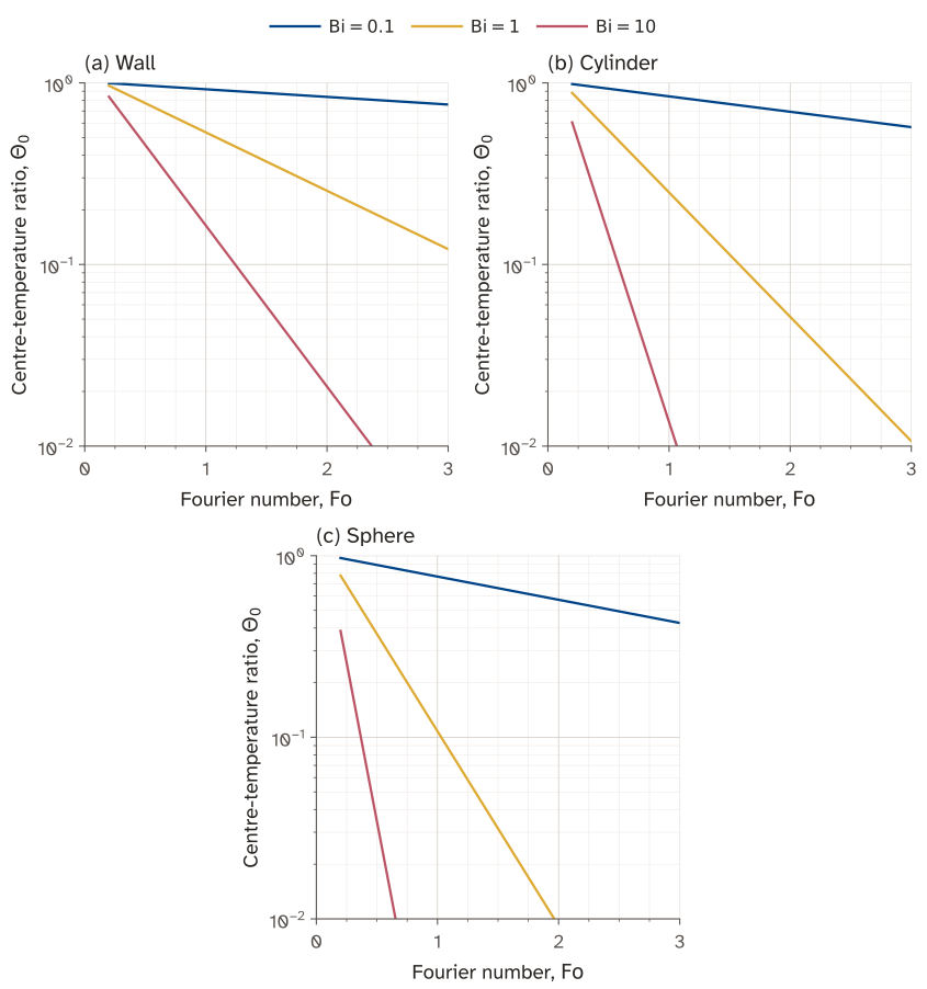
The one-term curves start at Fo =0.2$\mathrm{Fo}=0.2$.

5.5 Cylinder and sphere solutions and charts

The one-term cylinder and sphere solutions share the centre time factor in Eq. 18, but use Fo =𝛼𝑡/𝑟2𝑜$\mathrm{Fo}=\alpha t/r_o^2$ and their own roots and coefficients. With 𝑅 =𝑟/𝑟𝑜$R=r/r_o$, their position functions are

Θ𝑐(𝑅,𝑡)=Θ0,𝑐(𝑡)𝐽0(𝜆1𝑅)$$\Theta_c(R,t)=\Theta_{0,c}(t)J_0(\lambda_1R)$$(24)

Θ𝑠(𝑅,𝑡)=Θ0,𝑠(𝑡)sin⁡(𝜆1𝑅)𝜆1𝑅$$\Theta_s(R,t)=\Theta_{0,s}(t) \frac{\sin(\lambda_1R)}{\lambda_1R}$$(25)

At the centre use the limit sin⁡𝑧/𝑧 →1$\sin z/z\to1$, avoiding division by zero. Every shape function equals one at its centre and has zero centre gradient. The cylinder is long enough for end losses to be negligible. A short cylinder needs both axial and radial factors, as in classroom example 4.

The centre charts on source slides 23 and 25 use the same logarithmic excess axis and 1/Bi$1/\mathrm{Bi}$ curve labels as the wall chart. Source slides 24 and 26 show position ratios and cumulative-energy fractions. Their computed replacements are Figure 3 and Figure 4, with the heat fractions obtained from volume averages,

¯¯¯¯¯Θ𝑐=Θ0,𝑐2𝐽1(𝜆1)𝜆1$$\overline\Theta_c=\Theta_{0,c} \frac{2J_1(\lambda_1)}{\lambda_1}$$(26)

¯¯¯¯¯Θ𝑠=Θ0,𝑠3(sin⁡𝜆1−𝜆1cos⁡𝜆1)𝜆31$$\overline\Theta_s=\Theta_{0,s} \frac{3(\sin\lambda_1-\lambda_1\cos\lambda_1)}{\lambda_1^3}$$(27)

Use

𝐸𝐸∞=1−¯¯¯¯¯Θ$$\frac{E}{E_\infty}=1-\overline\Theta$$

for each geometry. For the same geometry length, Biot and Fourier numbers, a sphere responds faster than a cylinder, which responds faster than a wall. Their surface area per volume increases in that order. These comparisons need matching dimensionless groups; size or chart-axis limits alone do not establish a universal ranking.

Figure 4: Original wall, cylinder and sphere position-ratio curves at Biot numbers 0.1, 1 and 10, each beginning at one at the centre and falling toward its surface.

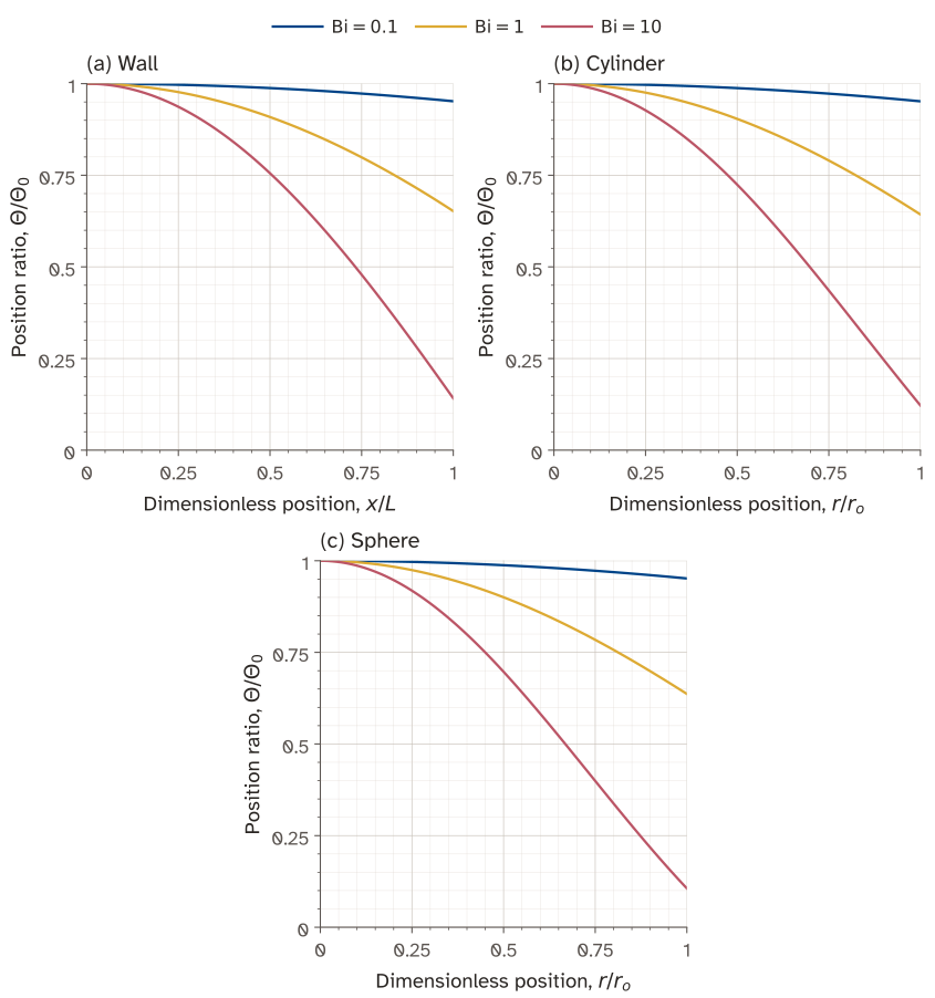
The horizontal coordinate is 𝑥/𝐿$x/L$ for the wall and 𝑟/𝑟𝑜$r/r_o$ for the cylinder and sphere. Multiply the plotted position ratio by Θ0$\Theta_0$.

5.6 Classroom example 3: insulated brick wall

Cooling an insulated brick wall

A flat wall of fire-clay brick (0.5 m thick) initially has a uniform temperature of 200 K. One of its faces is suddenly exposed to hot gas at 1200 K. If the heat transfer coefficient on the hot side is 7.38 W/(m2⋅K)$7.38\ \mathrm{W/(m^2\cdot K)}$ and the other face of the wall is insulated, determine:

• The time it takes for the centre of the wall to reach 600 K
• The temperature of the insulated wall at the time evaluated in (a)

Properties of fire-clay brick:

• 𝑘 =1.125 W/(m K)$k=1.125\ \mathrm{W/(m\,K)}$
• 𝐶𝑝 =919 J/(kg K)$C_p=919\ \mathrm{J/(kg\,K)}$
• 𝜌 =2310 kg/m3$\rho=2310\ \mathrm{kg/m^3}$

Worked solution

The insulated face has zero normal temperature gradient. Reflecting the brick about that face produces a symmetric wall heated from both sides.

Figure 5: A brick wall heated by gas on one face and insulated on the other. Reflection makes the insulated face the symmetry plane of a wall twice as thick.

Data

Quantity	Value
Real brick thickness	𝑏 =0.50 m$b=0.50\ \mathrm m$
Initial temperature	𝑇𝑖 =200 K$T_i=200\ \mathrm K$
Gas temperature	𝑇∞ =1200 K$T_\infty=1200\ \mathrm K$
Heat transfer coefficient	ℎ =7.38 W m−2 K−1$h=7.38\ \mathrm{W\,m^{-2}\,K^{-1}}$
Brick conductivity	𝑘 =1.125 W m−1 K−1$k=1.125\ \mathrm{W\,m^{-1}\,K^{-1}}$
Brick density	𝜌 =2310 kg m−3$\rho=2310\ \mathrm{kg\,m^{-3}}$
Specific heat capacity	𝐶𝑝 =919 J kg−1 K−1$C_p=919\ \mathrm{J\,kg^{-1}\,K^{-1}}$
Reflected-wall half-thickness	𝐿 =0.50 m$L=0.50\ \mathrm m$
Physical brick-centre position	𝑥 =0.25 m$x=0.25\ \mathrm m$, 𝑋 =𝑥/𝐿 =0.5$X=x/L=0.5$
Target temperature at the brick centre	𝑇 =600 K$T=600\ \mathrm K$

Measure position from the insulated face. Reflection makes that face the midplane of the equivalent wall.

Assumptions

• Uniform initial temperature.
• Unidirectional conduction normal to the wall.
• Perfect insulation at the rear face.
• Constant material properties, gas temperature and heat transfer coefficient.
• No internal heat generation.
• Radiation is neglected.

Calculations

The insulated face obeys ∂𝑇/∂𝑥 =0$\partial T/\partial x=0$, which is the symmetry condition of the finite-wall solution. First calculate the diffusivity:

𝛼=𝑘𝜌𝐶𝑝=1.1252310(919)=5.2992×10−7 m2 s−1$$\alpha=\frac{k}{\rho C_p} =\frac{1.125}{2310(919)}=5.2992\times10^{-7}\ \mathrm{m^2\,s^{-1}}$$

The wall Biot number is

Bi=ℎ𝐿𝑘=7.38(0.50)1.125=3.28$$\mathrm{Bi}=\frac{hL}{k}=\frac{7.38(0.50)}{1.125}=3.28$$

For this one-sided wall, 𝑉/𝐴𝑠 =0.50 m$V/A_s=0.50\ \mathrm{m}$ also. The Biot number is well above 0.1, so a spatial temperature profile is needed. The one-term wall solution from Eq. 18 is

Θ(𝑋,𝑡)=𝐴1𝑒−𝜆21Focos⁡(𝜆1𝑋),Fo=𝛼𝑡𝐿2$$\Theta(X,t)=A_1e^{-\lambda_1^2\mathrm{Fo}}\cos(\lambda_1X), \qquad \mathrm{Fo}=\frac{\alpha t}{L^2}$$

The eigenvalue relation Eq. 15, 𝜆1tan⁡𝜆1 =Bi$\lambda_1\tan\lambda_1=\mathrm{Bi}$, gives 𝜆1 =1.21582$\lambda_1=1.21582$. Substituting that root into the coefficient relation gives

𝐴1=4sin⁡𝜆12𝜆1+sin⁡(2𝜆1)=4sin⁡(1.21582)2(1.21582)+sin⁡(2.43164)=1.21638$$A_1=\frac{4\sin\lambda_1}{2\lambda_1+\sin(2\lambda_1)} =\frac{4\sin(1.21582)}{2(1.21582)+\sin(2.43164)}=1.21638$$

At the real brick centre, the requested temperature corresponds to

Θ(0.5,𝑡)=600−1200200−1200=0.600$$\Theta(0.5,t)=\frac{600-1200}{200-1200}=0.600$$

The value 0.600$0.600$ applies at the physical centre of the brick, 𝑥 =0.25 m$x=0.25\ \mathrm m$ or 𝑋 =0.5$X=0.5$. The reference position for the symmetric wall solution is 𝑥 =0$x=0$, at the insulated face. This is the centre of the equivalent reflected wall, so it is a different location from the physical centre of the brick.

At 𝑋 =0$X=0$, the cosine factor is one and the one-term solution gives Θ0 =Θ(0,𝑡) =𝐴1𝑒−𝜆21Fo$\Theta_0=\Theta(0,t)=A_1e^{-\lambda_1^2\mathrm{Fo}}$. At the physical brick centre, it therefore gives Θ(0.5,𝑡) =Θ0cos⁡(𝜆1/2)$\Theta(0.5,t)=\Theta_0\cos(\lambda_1/2)$. Divide by this cosine factor to find the dimensionless temperature at the insulated face:

Θ0=Θ(0.5,𝑡)cos⁡(𝜆12)=0.600cos⁡(1.215822)=0.73096$$\Theta_0=\frac{\Theta(0.5,t)}{\cos\left(\frac{\lambda_1}{2}\right)} =\frac{0.600}{\cos\left(\frac{1.21582}{2}\right)}=0.73096$$

Thus 0.600$0.600$ and 0.73096$0.73096$ are dimensionless temperatures at different positions at the same time. The value 0.73096$0.73096$ is the insulated-face reference value needed to find the elapsed time.

Use

Θ0=𝐴1𝑒−𝜆21Fo$$\Theta_0=A_1e^{-\lambda_1^2\mathrm{Fo}}$$

to find the elapsed time:

Fo=ln⁡(𝐴1Θ0)𝜆21=ln⁡(1.216380.73096)1.215822=0.34452$$\mathrm{Fo}=\frac{\ln\left(\frac{A_1}{\Theta_0}\right)}{\lambda_1^2} =\frac{\ln\left(\frac{1.21638}{0.73096}\right)}{1.21582^2}=0.34452$$(28)

Since Fo >0.2$\mathrm{Fo}>0.2$, the one-term approximation is appropriate. Convert this dimensionless time to seconds:

𝑡=Fo𝐿2𝛼=0.34452(0.50)25.2992×10−7=1.6253×105 s=45.1 h$$t=\frac{\mathrm{Fo}L^2}{\alpha} =\frac{0.34452(0.50)^2}{5.2992\times10^{-7}} =1.6253\times10^5\ \mathrm{s}=45.1\ \mathrm{h}$$

At the insulated face, 𝑋 =0$X=0$ and the cosine factor is one. Its temperature is

𝑇0=𝑇∞+Θ0(𝑇𝑖−𝑇∞)=1200+0.73096(200−1200)=469.0 K$$T_0=T_\infty+\Theta_0(T_i-T_\infty) =1200+0.73096(200-1200)=469.0\ \mathrm{K}$$

The insulated face is colder than the brick centre because heat enters from the opposite face. The ordering 200 <𝑇0 <600 <1200 K$200<T_0<600<1200\ \mathrm{K}$ is consistent with one-sided heating. Constant properties over this temperature range are an idealisation of the classroom model.

Answer

The brick centre reaches 600 K$600\ \mathrm{K}$ after approximately 45.1 h$45.1\ \mathrm{h}$. At that time, the insulated face is at 469 K$469\ \mathrm{K}$.

5.7 Classroom example 4: short steel cylinder

Cooling a short steel cylinder

A steel cylinder (𝐷 =30.5 cm$D=30.5\ \mathrm{cm}$, 𝐿 =61 cm$L=61\ \mathrm{cm}$) is initially at 645 K. It is immersed in an oil bath with a constant temperature of 310K. If the convection heat transfer coefficient at the steel surface is 34 W/(m2⋅K)$34\ \mathrm{W/(m^2\cdot K)}$, determine the temperatures at the following locations:

• at the centre of the cylinder after 1 hour?
• at the centre of the top surface of the cylinder?

Properties of steel:

• 𝑘 =42.9 W/(m K)$k=42.9\ \mathrm{W/(m\,K)}$
• 𝐶𝑝 =473 J/(kg K)$C_p=473\ \mathrm{J/(kg\,K)}$
• 𝜌 =7820 kg/m3$\rho=7820\ \mathrm{kg/m^3}$

Worked solution

An axial section identifies the two requested points and the two directions of conduction.

Data

Quantity	Value
Cylinder diameter	𝐷 =0.305 m$D=0.305\ \mathrm m$
Full cylinder length	𝐿 =0.610 m$L=0.610\ \mathrm m$
Half-length for the plane-wall factor	𝐿𝑤 =0.305 m$L_w=0.305\ \mathrm m$
Cylinder radius	𝑟𝑜 =0.1525 m$r_o=0.1525\ \mathrm m$
Initial temperature	𝑇𝑖 =645 K$T_i=645\ \mathrm K$
Oil temperature	𝑇∞ =310 K$T_\infty=310\ \mathrm K$
Heat transfer coefficient	ℎ =34 W m−2 K−1$h=34\ \mathrm{W\,m^{-2}\,K^{-1}}$
Steel conductivity	𝑘 =42.9 W m−1 K−1$k=42.9\ \mathrm{W\,m^{-1}\,K^{-1}}$
Steel density	𝜌 =7820 kg m−3$\rho=7820\ \mathrm{kg\,m^{-3}}$
Specific heat capacity	𝐶𝑝 =473 J kg−1 K−1$C_p=473\ \mathrm{J\,kg^{-1}\,K^{-1}}$
Time for both requested temperatures	𝑡 =3600 s$t=3600\ \mathrm s$

Assumptions

• Uniform initial temperature.
• Axisymmetric conduction in both radial and axial directions.
• Constant material properties.
• Constant oil temperature and uniform heat transfer coefficient on all surfaces.
• No internal heat generation.
• Radiation is neglected.

Calculations

The ends cannot be neglected because the length is only twice the diameter. For a constant-property body with these separable boundary conditions, the short-cylinder excess-temperature ratio is the product of a wall factor and a long-cylinder factor:

Θ(𝑥,𝑟,𝑡)=Θ𝑤(𝑥,𝑡)Θ𝑐(𝑟,𝑡)$$\Theta(x,r,t)=\Theta_w(x,t)\Theta_c(r,t)$$(29)

Here 𝑥 =0$x=0$ is the axial midplane and 𝑟 =0$r=0$ is the axis. The product solves

∂𝑇∂𝑡=𝛼[∂2𝑇∂𝑥2+1𝑟∂∂𝑟(𝑟∂𝑇∂𝑟)],$$\frac{\partial T}{\partial t}=\alpha\left[\frac{\partial^2 T}{\partial x^2}+ \frac{1}{r}\frac{\partial}{\partial r}\left(r\frac{\partial T}{\partial r}\right)\right],$$

because each factor solves its own one-dimensional diffusion equation. The diffusivity is

𝛼=𝑘𝜌𝐶𝑝=42.97820(473)=1.1598×10−5 m2 s−1$$\alpha=\frac{k}{\rho C_p} =\frac{42.9}{7820(473)}=1.1598\times10^{-5}\ \mathrm{m^2\,s^{-1}}$$

Each factor needs its own Biot and Fourier numbers. For the wall factor,

Bi𝑤=ℎ𝐿𝑤𝑘=34(0.305)42.9=0.24172$$\mathrm{Bi}_w=\frac{hL_w}{k} =\frac{34(0.305)}{42.9}=0.24172$$Fo𝑤=𝛼𝑡𝐿2𝑤=1.1598×10−5(3600)0.3052=0.44884$$\mathrm{Fo}_w=\frac{\alpha t}{L_w^2} =\frac{1.1598\times10^{-5}(3600)}{0.305^2}=0.44884$$

For the cylindrical factor,

Bicyl=ℎ𝑟𝑜𝑘=34(0.1525)42.9=0.12086$$\mathrm{Bi}_{\mathrm{cyl}}=\frac{hr_o}{k} =\frac{34(0.1525)}{42.9}=0.12086$$Focyl=𝛼𝑡𝑟2𝑜=1.1598×10−5(3600)0.15252=1.7954$$\mathrm{Fo}_{\mathrm{cyl}}=\frac{\alpha t}{r_o^2} =\frac{1.1598\times10^{-5}(3600)}{0.1525^2}=1.7954$$

Both Fourier numbers exceed 0.2. Solving 𝜆𝑤tan⁡𝜆𝑤 =0.24172$\lambda_w\tan\lambda_w=0.24172$ and

𝜆𝑐𝐽1(𝜆𝑐)=0.12086𝐽0(𝜆𝑐)$$\lambda_cJ_1(\lambda_c)=0.12086J_0(\lambda_c)$$

gives 𝜆𝑤 =0.472701$\lambda_w=0.472701$ and 𝜆𝑐 =0.484321$\lambda_c=0.484321$. The corresponding coefficient relations, Eq. 17 and Eq. 21, give 𝐴𝑤 =1.03703$A_w=1.03703$ and 𝐴𝑐 =1.02960$A_c=1.02960$.

The wall centre factor is

Θ0,𝑤=𝐴𝑤𝑒−𝜆2𝑤Fo𝑤=1.03703𝑒−0.4727012(0.44884)=0.93807$$\Theta_{0,w}=A_we^{-\lambda_w^2\mathrm{Fo}_w} =1.03703e^{-0.472701^2(0.44884)}=0.93807$$

The cylinder centre factor is

Θ0,𝑐=𝐴𝑐𝑒−𝜆2𝑐Focyl=1.02960𝑒−0.4843212(1.7954)=0.67573$$\Theta_{0,c}=A_ce^{-\lambda_c^2\mathrm{Fo}_{\mathrm{cyl}}} =1.02960e^{-0.484321^2(1.7954)}=0.67573$$

At the body centre, both position factors are one. The product and resulting temperature are

Θ𝑂=Θ0,𝑤Θ0,𝑐=0.93807(0.67573)=0.63388$$\Theta_O=\Theta_{0,w}\Theta_{0,c} =0.93807(0.67573)=0.63388$$𝑇𝑂=𝑇∞+Θ𝑂(𝑇𝑖−𝑇∞)=310+0.63388(645−310)=522.4 K$$T_O=T_\infty+\Theta_O(T_i-T_\infty) =310+0.63388(645-310)=522.4\ \mathrm{K}$$

At the centre of the top face, 𝑥 =𝐿𝑤$x=L_w$ and 𝑟 =0$r=0$. The wall factor includes cos⁡𝜆𝑤$\cos\lambda_w$, while the radial position factor remains one:

Θ𝑇=Θ0,𝑤cos⁡𝜆𝑤 Θ0,𝑐=0.63388cos⁡(0.472701)=0.56437$$\Theta_T=\Theta_{0,w}\cos\lambda_w\,\Theta_{0,c} =0.63388\cos(0.472701)=0.56437$$

Convert the product to temperature:

𝑇𝑇=𝑇∞+Θ𝑇(𝑇𝑖−𝑇∞)=310+0.56437(645−310)=499.1 K$$T_T=T_\infty+\Theta_T(T_i-T_\infty) =310+0.56437(645-310)=499.1\ \mathrm{K}$$

The face centre is cooler than the body centre and both temperatures remain between the initial and bath temperatures. A position chart supplies a ratio relative to its own centre value. Multiplying a position ratio alone by the other centre factor would omit part of the cooling history.

Answer

After one hour, the body centre is at approximately 522 K$522\ \mathrm{K}$ and the centre of the top face is at approximately 499 K$499\ \mathrm{K}$.

5.8 Classroom example 5: egg model

Heating an egg

An egg, initially at a uniform temperature of 5 °C$5\ \degree\mathrm{C}$, is dropped into boiling water at 95 °C$95\ \degree\mathrm{C}$. Taking the convection heat transfer coefficient to be 1200 W/(m2⋅°C)$1200\ \mathrm{W/(m^2\cdot\degree\mathrm{C})}$, and approximating the egg to be a 5-cm diameter sphere, determine how long it will take for the centre of the egg to reach 70 °C$70\ \degree\mathrm{C}$.

Worked solution

Figure 6: The egg is modelled as a sphere heated by surrounding water. The requested temperature is at the centre, which can lag behind the surface.

Data

Quantity	Value
Model sphere diameter	𝐷 =0.050 m$D=0.050\ \mathrm m$
Initial temperature	𝑇𝑖 =5 °C$T_i=5\ \degree\mathrm C$
Target centre temperature	𝑇0 =70 °C$T_0=70\ \degree\mathrm C$
Water temperature	𝑇∞ =95 °C$T_\infty=95\ \degree\mathrm C$
Heat transfer coefficient	ℎ =1200 W m−2 K−1$h=1200\ \mathrm{W\,m^{-2}\,K^{-1}}$
Conductivity	𝑘 =0.627 W m−1 K−1$k=0.627\ \mathrm{W\,m^{-1}\,K^{-1}}$
Thermal diffusivity	𝛼 =0.151 ×10−6 m2 s−1$\alpha=0.151\times10^{-6}\ \mathrm{m^2\,s^{-1}}$

The conductivity and diffusivity come from the lecturer’s notes.

Assumptions

• Homogeneous spherical body with a uniform initial temperature.
• Radial conduction.
• Constant properties and heat transfer coefficient.
• Constant water temperature.
• No internal heat generation.
• Shell resistance and energy changes due to cooking are neglected.

Calculations

Test lumped capacitance using 𝐿𝑐 =𝐷/6$L_c=D/6$:

Bi𝑐=ℎ𝐷6𝑘=1200(0.050)6(0.627)=15.95$$\mathrm{Bi}_c=\frac{hD}{6k} =\frac{1200(0.050)}{6(0.627)}=15.95$$

The large Biot number rules out a uniform internal temperature. The sphere solution uses the radius 𝑟𝑜 =𝐷/2 =0.025 m$r_o=D/2=0.025\ \mathrm{m}$ instead:

Bi=ℎ𝑟𝑜𝑘=1200(0.025)0.627=47.85$$\mathrm{Bi}=\frac{hr_o}{k} =\frac{1200(0.025)}{0.627}=47.85$$

At the centre, the one-term solution is

Θ0=𝐴1𝑒−𝜆21Fo.$$\Theta_0=A_1e^{-\lambda_1^2\mathrm{Fo}}.$$

Its target value is

Θ0=𝑇0−𝑇∞𝑇𝑖−𝑇∞=70−955−95=0.27778$$\Theta_0=\frac{T_0-T_\infty}{T_i-T_\infty} =\frac{70-95}{5-95}=0.27778$$

The sphere eigenvalue relation Eq. 20 is 1 −𝜆1cot⁡𝜆1 =Bi$1-\lambda_1\cot\lambda_1=\mathrm{Bi}$. With Bi =47.85$\mathrm{Bi}=47.85$, its first root is 𝜆1 =3.07603$\lambda_1=3.07603$. The corresponding coefficient is

𝐴1=4(sin⁡𝜆1−𝜆1cos⁡𝜆1)2𝜆1−sin⁡(2𝜆1)=1.99588$$A_1=\frac{4(\sin\lambda_1-\lambda_1\cos\lambda_1)} {2\lambda_1-\sin(2\lambda_1)}=1.99588$$

Rearrange the centre-temperature relation to find the Fourier number:

Fo=ln⁡(𝐴1Θ0)𝜆21=ln⁡(1.995880.27778)3.076032=0.20842$$\mathrm{Fo}=\frac{\ln\left(\frac{A_1}{\Theta_0}\right)}{\lambda_1^2} =\frac{\ln\left(\frac{1.99588}{0.27778}\right)}{3.07603^2}=0.20842$$

This just exceeds 0.2, so the usual one-term criterion is satisfied. The time is

𝑡=Fo𝑟2𝑜𝛼=0.20842(0.025)20.151×10−6=863 s=14.4 min$$t=\frac{\mathrm{Fo}r_o^2}{\alpha} =\frac{0.20842(0.025)^2}{0.151\times10^{-6}} =863\ \mathrm{s}=14.4\ \mathrm{min}$$

A chart reading of Fo ≃0.20$\mathrm{Fo}\simeq0.20$ gives about 13.8 minutes, consistent with this estimate. The large Biot number means that internal conduction limits the response. Increasing the external coefficient has less effect than it would in a lumped body. Real eggs have a nonspherical shape and different internal regions, so the calculation is an idealised heating estimate.

Answer

The centre reaches 70 °C$70\,\degree\mathrm{C}$ after approximately 14 min$14\ \mathrm{min}$ in the spherical, constant-property model.

6 Non-lumped capacitance approach: semi-infinite medium

Semi-infinite medium

A semi-infinite medium is an idealised body that extends indefinitely in one direction away from its exposed surface. Its temperature approaches the initial temperature far from that surface. The model also approximates a finite body during the period when the surface temperature disturbance has not significantly reached another boundary.

6.1 Model and boundary conditions

A semi-infinite solid occupies 𝑥 ≥0$x\geq0$, with 𝑥$x$ measured inward from a plane surface. Its far field remains at the initial temperature over the time of interest. A finite body can use this approximation while the penetration distance √𝛼𝑡$\sqrt{\alpha t}$ is small relative to the distance 𝛿$\delta$ to an influential far boundary. A practical guide is 𝛼𝑡/𝛿2 <0.05$\alpha t/\delta^2<0.05$, followed by a check that the far boundary’s temperature change is acceptably small. This is a time-dependent condition, rather than a definition of a thick body.

The equation is still Eq. 11, with 𝑇(𝑥,0) =𝑇𝑖$T(x,0)=T_i$ and 𝑇(𝑥 →∞,𝑡) =𝑇𝑖$T(x\to\infty,t)=T_i$. Choose one surface condition. A prescribed-temperature surface has 𝑇(0,𝑡) =𝑇𝑠$T(0,t)=T_s$. Alternatively, a surface exposed to fluid has

𝑘[∂𝑇∂𝑥]𝑥=0=ℎ[𝑇(0,𝑡)−𝑇∞]$$k\left[\frac{\partial T}{\partial x}\right]_{x=0} =h[T(0,t)-T_\infty]$$(30)

The sign differs from Eq. 12 because 𝑥$x$ now points inward. For a prescribed-temperature problem, 𝑇𝑠$T_s$ is known. For a convection problem, 𝑇𝑠 =𝑇(0,𝑡)$T_s=T(0,t)$ is an unknown surface temperature determined by the flux balance. Choose the condition that matches the supplied information.

6.2 Error-function solution

Define the dimensionless depth

𝜉=𝑥2√𝛼𝑡.$$\xi=\frac{x}{2\sqrt{\alpha t}}.$$

This combines depth with the diffusion distance because the ideal body has no finite geometrical length. For a suddenly imposed constant 𝑇𝑠$T_s$,

𝑇(𝑥,𝑡)−𝑇𝑖𝑇𝑠−𝑇𝑖=erfc⁡(𝜉)$$\frac{T(x,t)-T_i}{T_s-T_i}=\operatorname{erfc}(\xi)$$(31)

The complementary error function is

erfc⁡(𝜉)=1−2√𝜋∫𝜉0𝑒−𝑢2 𝑑𝑢$$\operatorname{erfc}(\xi)= 1-\frac{2}{\sqrt\pi}\int_0^\xi e^{-u^2}\,du$$(32)

Here 𝑢$u$ is a dimensionless integration variable. At the surface erfc⁡(0) =1$\operatorname{erfc}(0)=1$ gives 𝑇𝑠$T_s$. At great depth erfc tends to zero and gives 𝑇𝑖$T_i$. A similarity substitution into Eq. 11 gives 𝑓′′ +2𝜉𝑓′ =0$f''+2\xi f'=0$. Integration gives 𝑓′$f'$ proportional to 𝑒−𝜉2$e^{-\xi^2}$; the surface and far-field values fix the normalisation in Eq. 32.

For convection, put

𝛽=ℎ√𝛼𝑡𝑘.$$\beta=\frac{h\sqrt{\alpha t}}{k}.$$

The fraction of the possible temperature change is

𝑇(𝑥,𝑡)−𝑇𝑖𝑇∞−𝑇𝑖=erfc⁡(𝜉)−𝐶(𝜉,𝛽)$$\frac{T(x,t)-T_i}{T_\infty-T_i} =\operatorname{erfc}(\xi)-C(\xi,\beta)$$(33)

𝐶(𝜉,𝛽)=𝑒2𝛽𝜉+𝛽2erfc⁡(𝜉+𝛽)$$C(\xi,\beta)=e^{2\beta\xi+\beta^2} \operatorname{erfc}(\xi+\beta)$$(34)

𝛽$\beta$ is a Biot number based on the growing penetration distance. Finite ℎ$h$ reduces the temperature change through the positive correction 𝐶$C$. In the infinite-ℎ$h$ limit the correction tends to zero and Eq. 31 follows with 𝑇𝑠 =𝑇∞$T_s=T_\infty$. Evaluate the correction or its relative size when deciding whether to neglect it. For example, at the surface and 𝛽 =2$\beta=2$, the correction is about 0.255. The prescribed-temperature approximation would therefore overpredict the fractional surface temperature change by 0.255 at that instant. For large arguments a scaled complementary error function avoids overflow when evaluating the exponential times erfc.

For the same semi-infinite solid and prescribed surface-temperature step, how does the depth of a fixed fractional temperature change vary when time increases by a factor of four?

• It stays the same.
• It increases by a factor of four.
• It decreases by a factor of two.
• It increases by a factor of two. ✓

Explanation

For the same fractional temperature change, the similarity variable stays constant:

𝜂=𝑥2√𝛼𝑡$$\eta=\frac{x}{2\sqrt{\alpha t}}$$

With diffusivity unchanged,

𝑥2𝑥1=√𝑡2𝑡1=√4=2$$\frac{x_2}{x_1}=\sqrt{\frac{t_2}{t_1}}=\sqrt{4}=2$$

The depth doubles. The semi-infinite approximation must still be valid at the later time.

6.3 Evaluating the semi-infinite solution

Figure 7: Calculated semi-infinite temperature-change curves for penetration Biot numbers 0.5, 2 and infinity. The infinite limit represents a prescribed surface temperature.

The curves evaluate Eq. 33 and Eq. 31. For comparison, erfc⁡(0.5) =0.479500$\operatorname{erfc}(0.5)=0.479500$, erfc⁡(1) =0.157299$\operatorname{erfc}(1)=0.157299$ and erfc⁡(2) =0.004678$\operatorname{erfc}(2)=0.004678$.

6.4 Classroom example 6: soil frost depth

Soil frost depth

What minimum burial depth would you recommend to avoid freezing under conditions for which the soil, initially at a uniform temperature of 15 °C$15\ \degree\mathrm{C}$, is subjected to a constant surface temperature of −10 °C$-10\ \degree\mathrm{C}$ for 3 months?

Properties of soil:

• 𝑘 =0.52 W/(m⋅K)$k=0.52\ \mathrm{W/(m\cdot K)}$
• 𝐶𝑝 =1840 J/(kg⋅K)$C_p=1840\ \mathrm{J/(kg\cdot K)}$
• 𝜌 =2050 kg/m3$\rho=2050\ \mathrm{kg/m^3}$

Worked solution

Measure depth downwards from the cold ground surface. The pipe must lie below the calculated zero-degree isotherm.

Data

Quantity	Value
Initial soil temperature	𝑇𝑖 =15 °C$T_i=15\ \degree\mathrm C$
Prescribed surface temperature	𝑇𝑠 = −10 °C$T_s=-10\ \degree\mathrm C$
Temperature at the required depth	𝑇 =0 °C$T=0\ \degree\mathrm C$
Elapsed time	𝑡 =90 days$t=90\ \mathrm{days}$
Soil conductivity	𝑘 =0.52 W m−1 K−1$k=0.52\ \mathrm{W\,m^{-1}\,K^{-1}}$
Soil density	𝜌 =2050 kg m−3$\rho=2050\ \mathrm{kg\,m^{-3}}$
Specific heat capacity	𝐶𝑝 =1840 J kg−1 K−1$C_p=1840\ \mathrm{J\,kg^{-1}\,K^{-1}}$

For this calculation, take three months as 90 days.

Assumptions

• Uniform initial soil temperature.
• Unidirectional conduction normal to a plane ground surface.
• Semi-infinite soil depth over the time considered.
• Constant thermal properties.
• Constant prescribed surface temperature.
• No internal heat generation.
• Soil moisture phase change is neglected.

Calculations

The surface temperature is supplied directly, so use the prescribed-temperature semi-infinite solution rather than a convection boundary condition. The thermal diffusivity is

𝛼=𝑘𝜌𝐶𝑝=0.522050(1840)=1.3786×10−7 m2 s−1$$\alpha=\frac{k}{\rho C_p} =\frac{0.52}{2050(1840)}=1.3786\times10^{-7}\ \mathrm{m^2\,s^{-1}}$$

Convert the duration to seconds:

𝑡=90(24)(3600)=7.776×106 s$$t=90(24)(3600)=7.776\times10^6\ \mathrm{s}$$

The diffusion distance provides a useful estimate before solving for depth:

√𝛼𝑡=√1.3786×10−7(7.776×106)=1.0354 m$$\sqrt{\alpha t}=\sqrt{1.3786\times10^{-7}(7.776\times10^6)} =1.0354\ \mathrm{m}$$

The temperature relation from Eq. 31 is

𝑇(𝑥,𝑡)−𝑇𝑖𝑇𝑠−𝑇𝑖=erfc⁡(𝑥2√𝛼𝑡)$$\frac{T(x,t)-T_i}{T_s-T_i} =\operatorname{erfc}\left(\frac{x}{2\sqrt{\alpha t}}\right)$$

At the limiting temperature of 0 °C$0\,\degree\mathrm{C}$,

erfc⁡(𝜉)=0−15−10−15=0.600$$\operatorname{erfc}(\xi)=\frac{0-15}{-10-15}=0.600$$

Inverting the complementary error function gives 𝜉 =0.370807$\xi=0.370807$. The corresponding depth is

𝑥=2𝜉√𝛼𝑡=2(0.370807)(1.0354)=0.7679 m$$x=2\xi\sqrt{\alpha t}=2(0.370807)(1.0354)=0.7679\ \mathrm{m}$$

Temperature increases with depth during cooling, so a pipe deeper than this isotherm remains above 0 °C$0\,\degree\mathrm{C}$ within the model. The calculated depth is consistent with the metre-scale diffusion distance. The far boundary must be well below the disturbed region for the semi-infinite approximation to hold.

Soil moisture releases latent heat on freezing, which this calculation omits. Snow cover and a changing surface temperature would also alter the temperature profile. The result is a classroom estimate based on the specified temperature history.

Answer

The 0 °C$0\,\degree\mathrm{C}$ isotherm reaches approximately 0.77 m$0.77\ \mathrm{m}$. A burial depth of at least 0.8 m$0.8\ \mathrm{m}$ lies below it in this model; 1 m$1\ \mathrm{m}$ provides a larger margin.

A thick solid is exposed to fluid through a finite convection coefficient. Its disturbance has not reached the far boundary. Which surface condition should its early-time model use?

• Always set the solid surface temperature equal to the fluid temperature.
• Use convection at the surface, unless there is a reason to treat its temperature as fixed. ✓
• Set the surface equal to the fluid temperature and also require zero heat flux.
• No surface condition is needed for a semi-infinite solid.

Explanation

The semi-infinite approximation means that the temperature change has not yet reached the far boundary. Heat still has to cross the fluid film at the exposed surface:

𝑞into solid=ℎ(𝑇∞−𝑇𝑠)$$q_{\mathrm{into\ solid}}=h(T_\infty-T_s)$$

Keep this convection condition for finite resistance. Setting the solid surface equal to the fluid temperature is an additional approximation that needs its own justification.

7 Additional examples

Centre temperature and energy released by a cooling slab

A large slab of full thickness 0.100 m starts uniformly at 200 degrees Celsius. Both broad faces cool in fluid at 20 degrees Celsius with ℎ =20$h=20$ W m⁻² K⁻¹. Use 𝑘 =1.0$k=1.0$ W m⁻¹ K⁻¹, 𝜌 =2000$\rho=2000$ kg m⁻³ and 𝐶𝑝 =1000$C_p=1000$ J kg⁻¹ K⁻¹. Neglect edges, radiation and property variation.

After 30 minutes, find the centre, surface and volume-average temperatures, and the energy released per square metre of slab plan area. For the plane-wall one-term solution at Bi =1$\mathrm{Bi}=1$, use 𝜆1 =0.860334$\lambda_1=0.860334$ and 𝐴1 =1.11913$A_1=1.11913$. Check that this approximation is appropriate.

Worked solution

Figure 8: Both slab faces cool under the same conditions. The solution uses half-thickness L, measured from the symmetry plane to either exposed surface.

Data

Quantity	Value
Full slab thickness	2𝐿 =0.100 m$2L=0.100\ \mathrm m$
Half-thickness	𝐿 =0.050 m$L=0.050\ \mathrm m$
Initial temperature	𝑇𝑖 =200 °C$T_i=200\ \degree\mathrm C$
Fluid temperature	𝑇∞ =20 °C$T_\infty=20\ \degree\mathrm C$
Cooling time	𝑡 =1800 s$t=1800\ \mathrm s$
Heat transfer coefficient	ℎ =20 W m−2 K−1$h=20\ \mathrm{W\,m^{-2}\,K^{-1}}$
Conductivity	𝑘 =1.0 W m−1 K−1$k=1.0\ \mathrm{W\,m^{-1}\,K^{-1}}$
Density	𝜌 =2000 kg m−3$\rho=2000\ \mathrm{kg\,m^{-3}}$
Specific heat capacity	𝐶𝑝 =1000 J kg−1 K−1$C_p=1000\ \mathrm{J\,kg^{-1}\,K^{-1}}$
Supplied first eigenvalue	𝜆1 =0.860334$\lambda_1=0.860334$
Supplied first coefficient	𝐴1 =1.11913$A_1=1.11913$

Assumptions

• Uniform initial temperature.
• Unidirectional conduction through the slab thickness.
• Identical convection conditions on both broad faces.
• Constant properties, fluid temperature and heat transfer coefficient.
• Edge heat transfer and radiation are neglected.
• No internal heat generation.

Calculations

Both broad faces transfer heat. If 𝐴plan$A_{\mathrm{plan}}$ is the area of one face, 𝑉 =2𝐿𝐴plan$V=2LA_{\mathrm{plan}}$ and 𝐴𝑠 =2𝐴plan$A_s=2A_{\mathrm{plan}}$. Therefore

𝐿𝑐=𝑉𝐴𝑠=𝐿=0.050 m.$$L_c=\frac{V}{A_s}=L=0.050\ \mathrm{m}.$$

The Biot number is

Bi𝑐=ℎ𝐿𝑐𝑘=20(0.050)1.0=1.0$$\mathrm{Bi}_c=\frac{hL_c}{k}=\frac{20(0.050)}{1.0}=1.0$$

Lumped capacitance is unsuitable. Use the spatial wall solution, with 𝑥 =0$x=0$ at the midplane. First calculate the diffusivity:

𝛼=𝑘𝜌𝐶𝑝=1.02000(1000)=5.00×10−7 m2 s−1$$\alpha=\frac{k}{\rho C_p} =\frac{1.0}{2000(1000)}=5.00\times10^{-7}\ \mathrm{m^2\,s^{-1}}$$

The Fourier number uses the half-thickness:

Fo=𝛼𝑡𝐿2=5.00×10−7(1800)0.0502=0.360$$\mathrm{Fo}=\frac{\alpha t}{L^2} =\frac{5.00\times10^{-7}(1800)}{0.050^2}=0.360$$

Since Fo >0.2$\mathrm{Fo}>0.2$, the one-term approximation is appropriate. The wall profile is

Θ=Θ0cos⁡(𝜆1𝑥𝐿),$$\Theta=\Theta_0\cos\left(\frac{\lambda_1x}{L}\right),$$

where

Θ=𝑇−𝑇∞𝑇𝑖−𝑇∞.$$\Theta=\frac{T-T_\infty}{T_i-T_\infty}.$$

Its centre value is

Θ0=𝐴1𝑒−𝜆21Fo=1.11913𝑒−0.8603342(0.360)=0.8574$$\Theta_0=A_1e^{-\lambda_1^2\mathrm{Fo}} =1.11913e^{-0.860334^2(0.360)}=0.8574$$

Convert the centre ratio to temperature:

𝑇𝑐=𝑇∞+Θ0(𝑇𝑖−𝑇∞)=20+0.8574(200−20)=174.3 °C$$T_c=T_\infty+\Theta_0(T_i-T_\infty) =20+0.8574(200-20)=174.3\,\degree\mathrm{C}$$

At either face, 𝑥/𝐿 =1$x/L=1$. The surface ratio and temperature are

Θ𝑠=Θ0cos⁡𝜆1=0.8574cos⁡(0.860334)=0.5592$$\Theta_s=\Theta_0\cos\lambda_1 =0.8574\cos(0.860334)=0.5592$$𝑇𝑠=𝑇∞+Θ𝑠(𝑇𝑖−𝑇∞)=20+0.5592(180)=120.6 °C$$T_s=T_\infty+\Theta_s(T_i-T_\infty) =20+0.5592(180)=120.6\,\degree\mathrm{C}$$

Stored energy depends on the volume-average temperature. Integrating the symmetric profile across the thickness gives

¯¯¯¯¯Θ=Θ0∫10cos⁡(𝜆1𝑋) 𝑑𝑋=Θ0sin⁡𝜆1𝜆1=0.8574sin⁡(0.860334)0.860334=0.7554$$\bar\Theta=\Theta_0\int_0^1\cos(\lambda_1X)\,dX =\Theta_0\frac{\sin\lambda_1}{\lambda_1} =0.8574\frac{\sin(0.860334)}{0.860334}=0.7554$$

The average temperature is therefore

¯¯¯¯𝑇=𝑇∞+¯¯¯¯¯Θ(𝑇𝑖−𝑇∞)=20+0.7554(180)=156.0 °C$$\bar T=T_\infty+\bar\Theta(T_i-T_\infty) =20+0.7554(180)=156.0\,\degree\mathrm{C}$$

The released energy equals the decrease in stored thermal energy. Per unit plan area,

𝐸out𝐴plan=𝜌𝐶𝑝(2𝐿)(𝑇𝑖−¯¯¯¯𝑇)=2000(1000)(0.100)(200−156.0)=8.80×106 J m−2$$\frac{E_{\mathrm{out}}}{A_{\mathrm{plan}}} =\rho C_p(2L)(T_i-\bar T) =2000(1000)(0.100)(200-156.0) =8.80\times10^6\ \mathrm{J\,m^{-2}}$$

This includes heat leaving both faces. The ordering 20 <𝑇𝑠 <¯¯¯¯𝑇 <𝑇𝑐 <200 °C$20<T_s<\bar T<T_c<200\,\degree\mathrm{C}$ is consistent with cooling from the surfaces. Using the centre temperature for the energy balance would underestimate the heat released, because most of the slab is cooler than its centre.

Answer

After 30 minutes, 𝑇𝑐 =174.3 °C$T_c=174.3\,\degree\mathrm{C}$, 𝑇𝑠 =120.6 °C$T_s=120.6\,\degree\mathrm{C}$ and ¯¯¯¯𝑇 =156.0 °C$\bar T=156.0\,\degree\mathrm{C}$. The energy released is 8.80 MJ m−2$8.80\ \mathrm{MJ\,m^{-2}}$ of plan area.

8 What you should now be able to calculate

Test the lumped assumption, calculate temperatures at specified positions and times, and check finite-body or semi-infinite approximations.

Practice: Workshop 6 for plate heating and spherical transients.

9 Report an error

Email Ranjeet Utikar with the title Transient heat conduction, the URL /heat-transport/transient-conduction/, and the equation or passage to check.

References

Bird, R. Byron, Warren E. Stewart, and Edwin N. Lightfoot. 2006. Transport Phenomena. Revised 2nd. John Wiley & Sons. https://www.wiley-vch.de/en/areas-interest/engineering/transport-phenomena-978-0-470-11539-8.

Çengel, Yunus A., and Afshin J. Ghajar. 2015. Heat and Mass Transfer: Fundamentals and Applications. 5th ed. McGraw-Hill Education. https://glencoe.mheducation.com/sites/0073398187/information_center_view0/application_chapters.html.

Shah, Milinkumar. n.d. “CHEN3001-TP: Heat Transport 2.” Curtin University. Unpublished.